When we go to work at the Mercator Telescope, 20% of the total observing time can be used for our own purposes. In the past this helped me to get additional spectra for my Kepler stars, but it also made it possible for me to help out my collaborators when they needed some extra observations. During my last observing run though, I spent a large portion of this time on making “pretty pictures” with the MAIA camera, resulting in a nice collection of outreach-ready images that the Institute of Astronomy can use in the future for PR. This post is a small how-to guide for making similar images.
1. Planning the observations
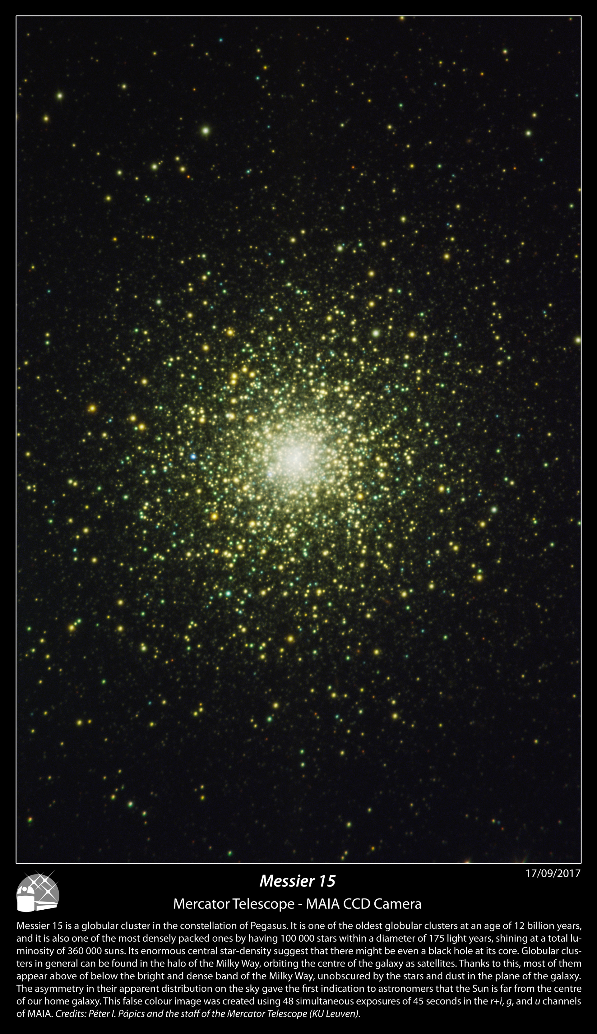
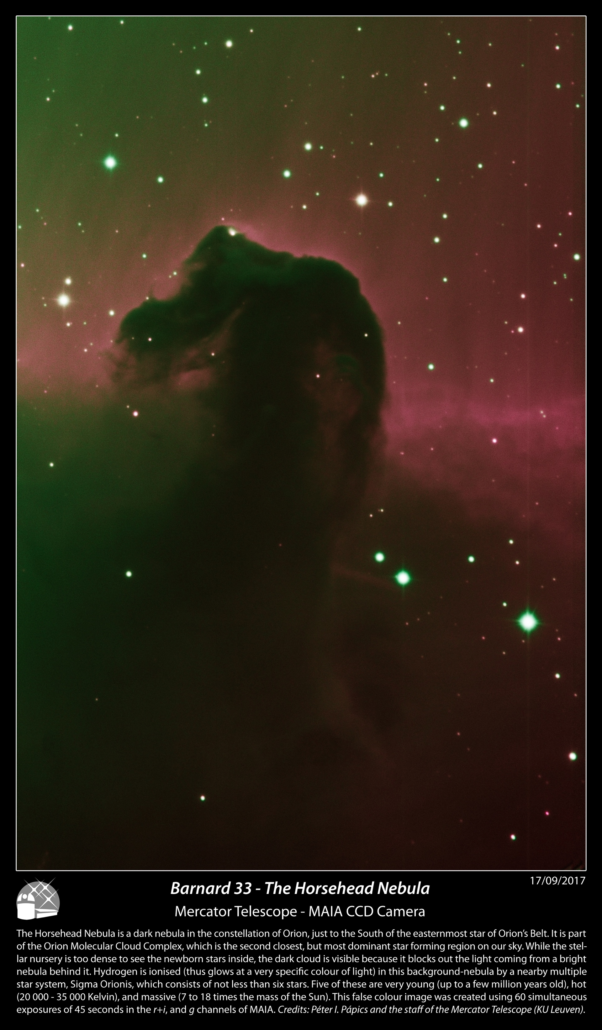
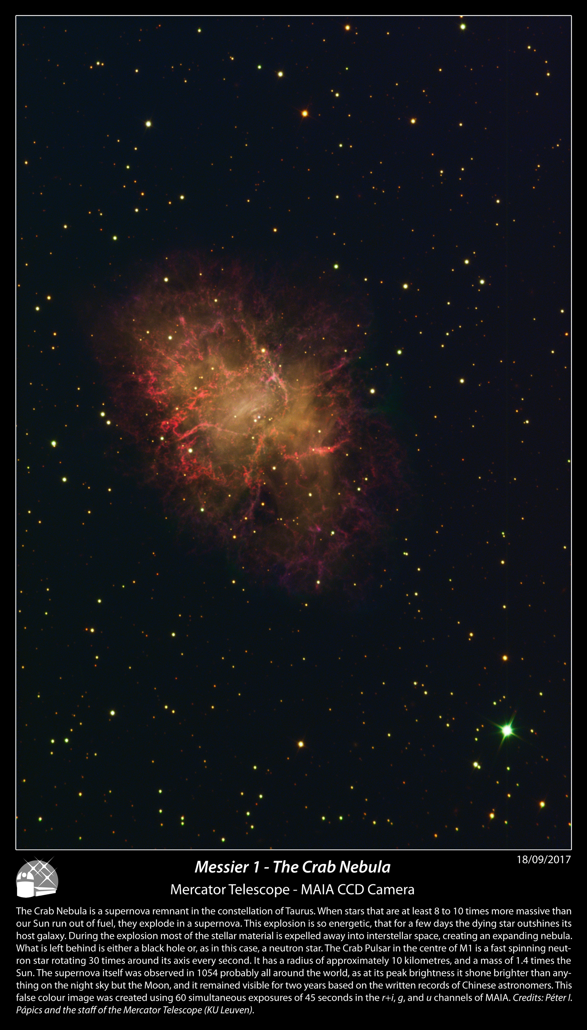
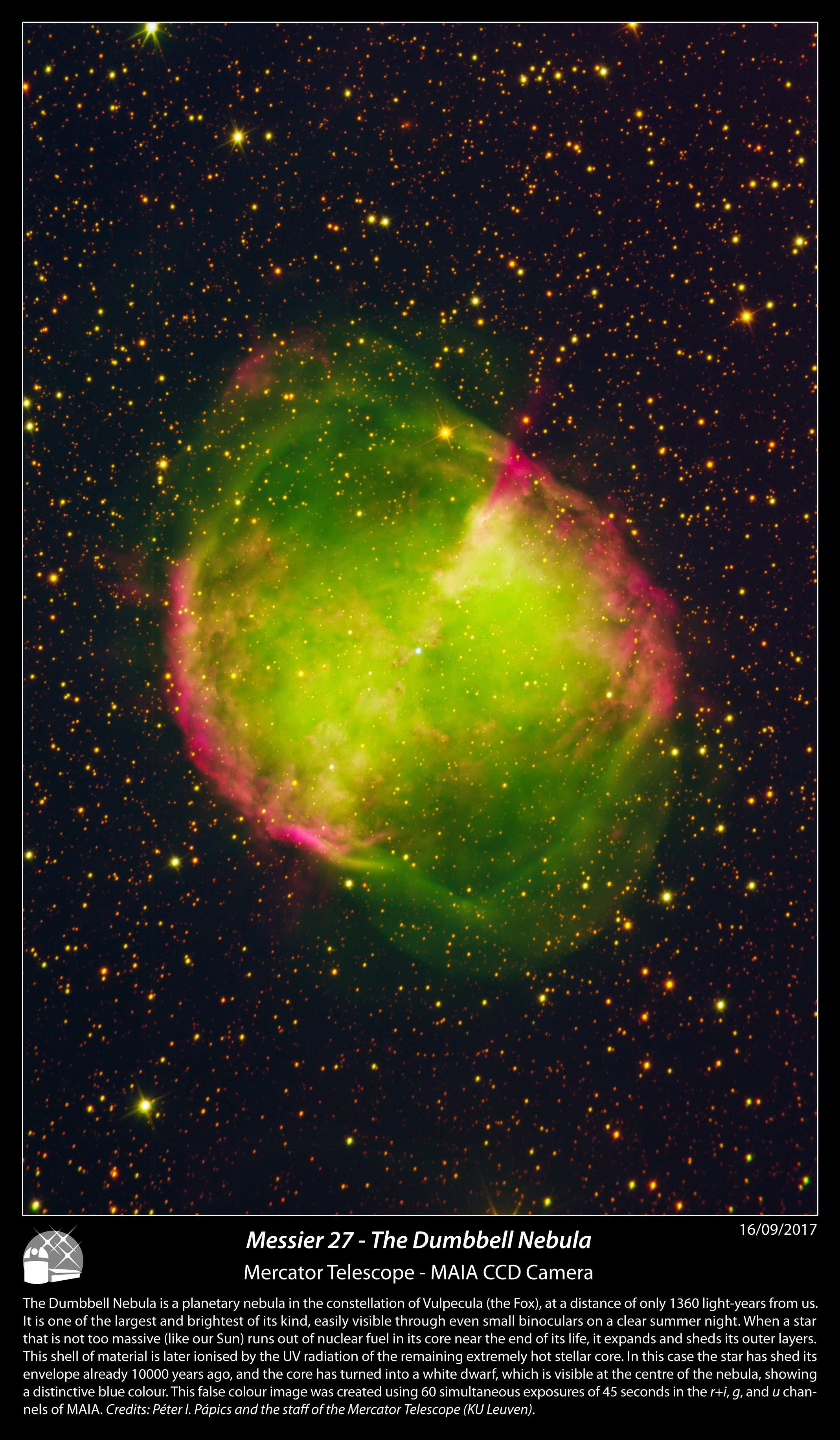
To be able to select a suitable target, you need to be familiar with the specifications of the instrument. MAIA is a simultaneous 3 channel frame-transfer CCD camera, meaning that as long as the exposure time is 44 seconds (it takes this long to read out one full frame without using windowing) or longer, it can take exposures continuously and simultaneously in three different channels. It has a chip size of 2k × 3k pixels, and a field of view of 9.4′ × 14.1′, which translates into a resolution of 0.275″/pixel. The three channels are r+i, g, and u (which can be though of as red, green, and blue, and they are labelled as R, G, and U in the system).
To select a target you also need to know the sky. You can use free software like Stellarium to see what objects are visible at a given time and position, just do not forget to actually set your location to the Roque de los Muchachos Observatory (and maybe install my Mercator panorama to really see what you would when standing in front of the observatory building on La Palma). If you want to search in a database, then the one of the Saguaro Astronomy Club is a good resource. You will want a target that is between 3′ and 9′ in size (or larger if you do not want to have the whole object in the field of view). 99% of targets this size will be perfectly suitable for MAIA, so you do not need to worry about their brightness.
You need to avoid bright stars in the field, because using an exposure time of 45 seconds stars that are brighter than 10-11 magnitudes (depending on the seeing conditions) will saturate the CCD and will cause vertical stripes on the final image. You can either use Stellarium, or the desktop client of Aladin to prepare the framing of your image, then record the central coordinate very precisely and use it later on for the pointing of the telescope. The pointing model of MAIA is spot in, so if your coordinate is precise, your target will be in the middle of the frame.
2. Imaging with MAIA
At the beginning of the night you need to take a set of calibration frames for MAIA too, most importantly sky flats. These are standard series, you can pick them from the Scheduler GUI, just pick the month, the time of the day (evening), and leave the default series of 10 U, and 10 R as they are fine like that. Start the sequence when the GUI says that there is ~40 minutes left until the start of the night, then the sky will be dark enough already for the U frames. Do not forget to stop the tracking of the telescope after pointing, this way stars will move across the field and their trails will be thrown out upon calculation a median flat field. You can take bias and dark frames too, or use the prescan area of the CCD to calculate these values (I do this, and for the pretty images, this is definitely satisfactory).
Do these kind of outreach observations preferably when there is a gap in available targets for the actual science programs, so you are not wasting valuable science time. For the object frames set frame transfer on (this puts a lower limit on the exposure time and thus on the brightness of the brightest unsaturated stars as already mentioned earlier, but saves a large amount of time). Focus the telescope. For pretty pictures a good focus is much more important than for time-series photometry! In the Focusing GIU start from thermal focus position minus 0.05 mm, do 3 measurements on both sides with a step of 0.02 mm (larger if seeing is worse), and keep an eye on the images in the ds9 window (use log scaling for better clarity) while the focus sequence is being done. Sometimes the fitted parabola in the GUI is not very precise (especially in U), but during the process you can easily see by eye when the sharpest – most circular – stars were achieved. Set that position in the focus GUI, then unselect the “thermal focus after each pointing” in the Scheduler GUI.
When setting up the exposures, use a series of 4-1-1 for U, G, and R. This means that by setting an exposure time of 45 seconds, you will get one U exposure of 4 × 45 (180) seconds, and four 45 second exposures of G and R each in one exposure repetition. There are some bad columns on the CCD especially in R, so to make life easier I suggest to use dithering, meaning that after a few exposure repetitions you need to move the telescope 3-5″ (or ~1 second) in RA (since the bad columns are along equal RA meridians), and you need to do this at least 2 times for one target. As a result later on when we sync up the frames based on the stars’ positions, the bad columns will not always fall on the same part of the sky, so calculating a median will get rid of them very easily. You do not need to have the guiding on during these observations, as tracking alone is perfectly good enough when the exposure times are so short.
My suggested setup is: 3 exposure groups (dithering of 3-5″ between these) of 5 repetitions each (3 × 5 × 1 U, and 3 × 5 × 4 G, and R frames), which adds up to a total exposure time of 2700 seconds per channel (in 20 and 60 subs of 180 and 45 seconds per channel, respectively). You can use the field rotator for better framing, but do not forget that if you set it to 90 degrees, then dithering needs to be in the declination direction instead of right ascension.
3. Data reduction
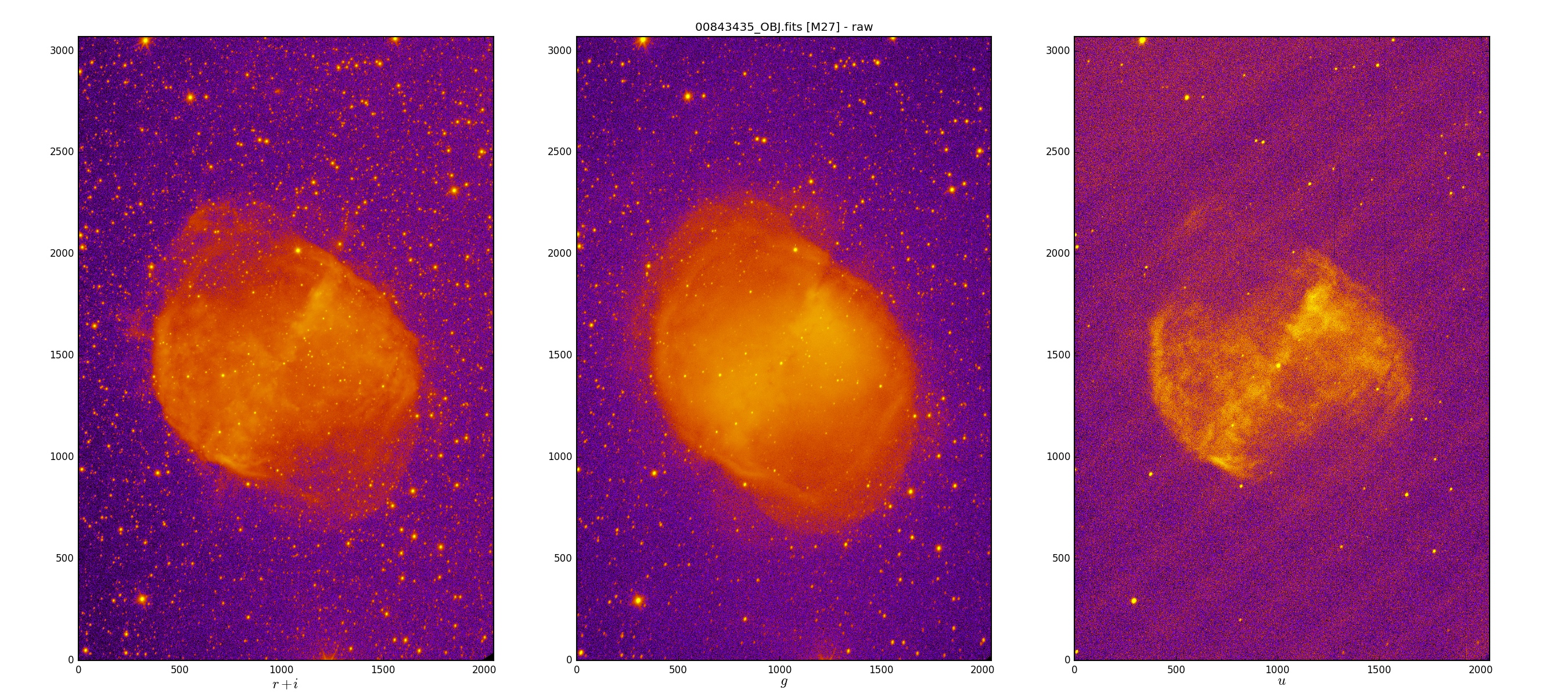
When the observations are done, we can start with the data reduction. Just like when working with science data, we first need to calibrate the object frames (to remove artefacts coming from the spatially non constant sensitivity of the CCD chip and dust in front of the detectors). You can do it with your own software/script, or you can simply use a python script I made to automate this step. The only thing you need to remember is that calibration needs to be done channel-by-channel, and that the MAIA fits files always contain three channels, but not always all three are useful. For example during sky flats some files will only contain U channel data, others only G and R. Similarly, object frames will most often only have data in the R and G channels, as only every fourth exposure will contain all three channels (since we set up the exposures this way).
If you want to use my script, just copy all *_FFS.fits and *_OBJ.fits files in the same folder where the reduceMAIA_PR.py file is, and run it in terminal simply by typing “python reduceMAIA_PR.py”. This will create a master flat frame for each channel, and three processed fits files for each OBJ file (one per channel). The script calculates the bias and dark currents from each object file’s prescan area, so it does not need *_BIAS.fits and *_DARK.fits calibration frames. Important note: do not use this script for science data reduction as it is, but use line 164 instead of line 163! I am “cheating” during the flat-fielding of the U channel, long story short, I had to do this to fully remove the remnants of the strong background pattern even at the very low signal level. I have ideas why the proper flat-fielding does not produce fully satisfactory results in the U channel without this “cheat”, but I don’t have time to test it out, and it already works fine enough for the purpose of making pretty images.
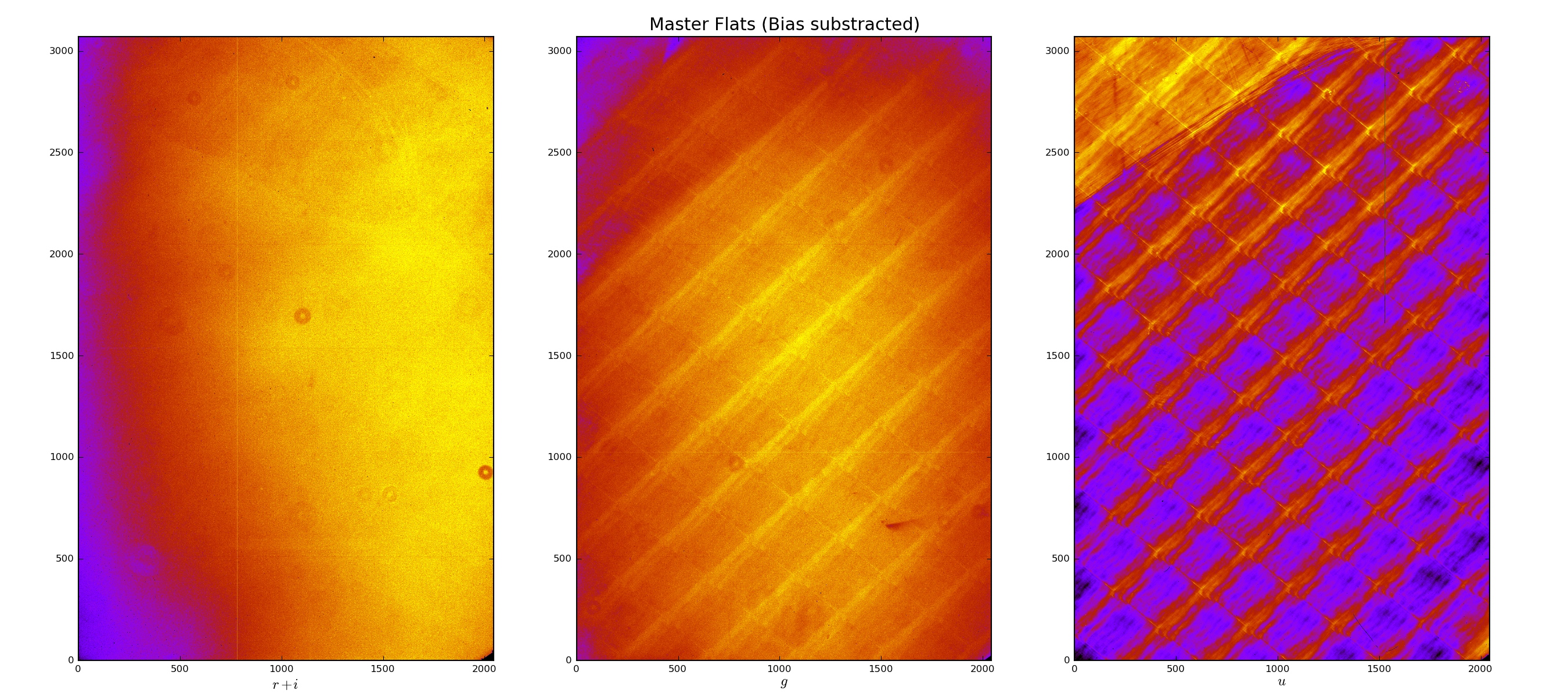
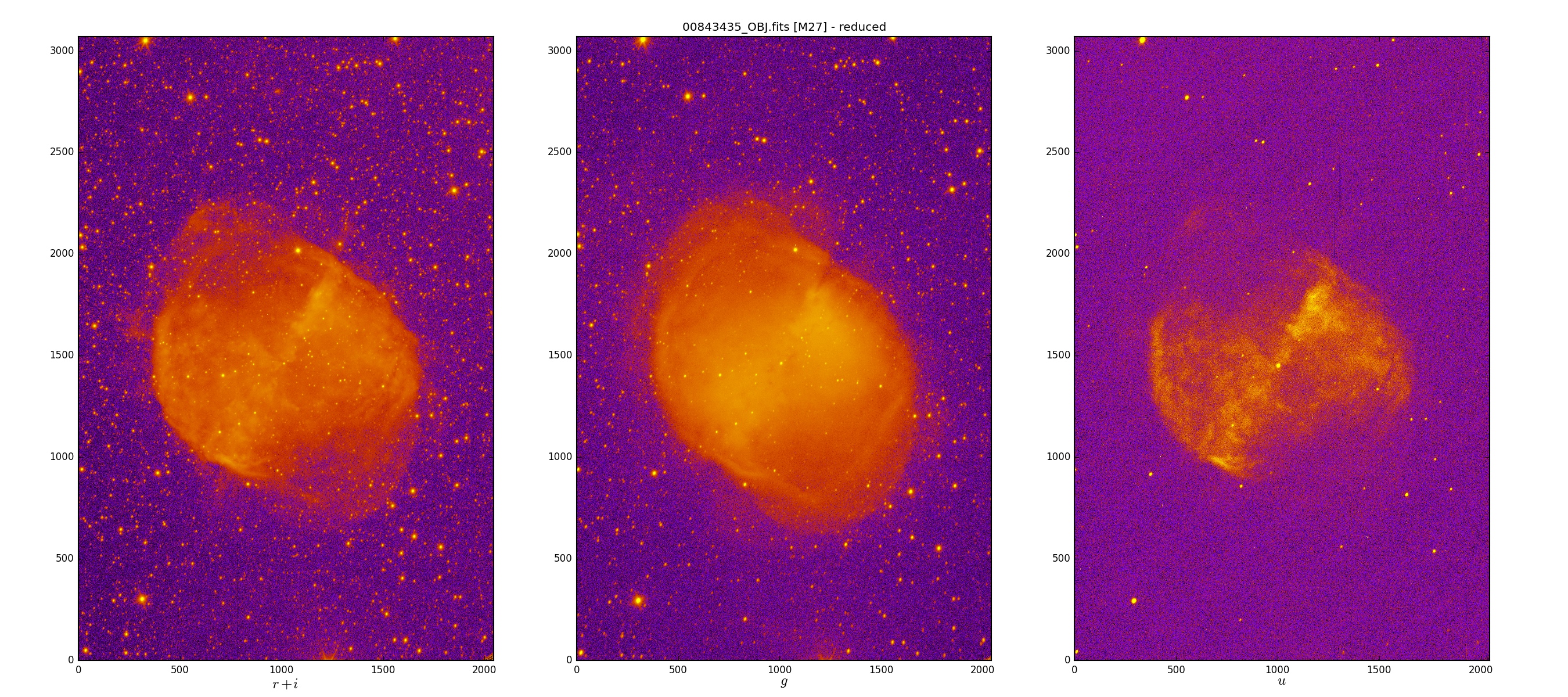
Here is a comparison of a raw OBJ frame, the master flat fields, and the calibrated exposures.
4. Image processing
So how do we get to a single colour image from these monochrome frames? The main purpose of taking 60 subs and not a single 2700 second exposure photo was a) lowering the noise, and b) avoiding saturation of the (brighter) stars. We need to integrate these subs (60 or 20, depending on the channel) together, then use the three master channels to create the colour composite. The main difficulty: the optical path to the three CCDs is different, so the stars in the three different channels are at slightly different positions, and it is not a linear transformation to go from one frame to another.
I use AstroPixelProcessor (APP) for the following steps, and since there is a 30 day fully-functional trial version, you can always download it when at the telescope to experiment with it during your observing run. It is a very self-explanatory software package with a good amount of on-line and in-software documentation/help available, so I am only going to summarise the steps of my workflow, instead of going into extensive detail.
Work plan per channel: find star positions (in APP: “Analyse Stars”; for U you should set the sigma to lower if it does not find enough stars), shift and transform images to a common frame (this is to correct for the dithering jumps and guiding shifts, in APP: “Register”; might have to set pattern recognition to triangles if there are too few stars in the frame), integrate separate frames together (in APP: “Integrate”; median for R to get rid of the bad columns, average with simple sigma clipping as outlier rejection for G, and U), save integrated image to a fits file.
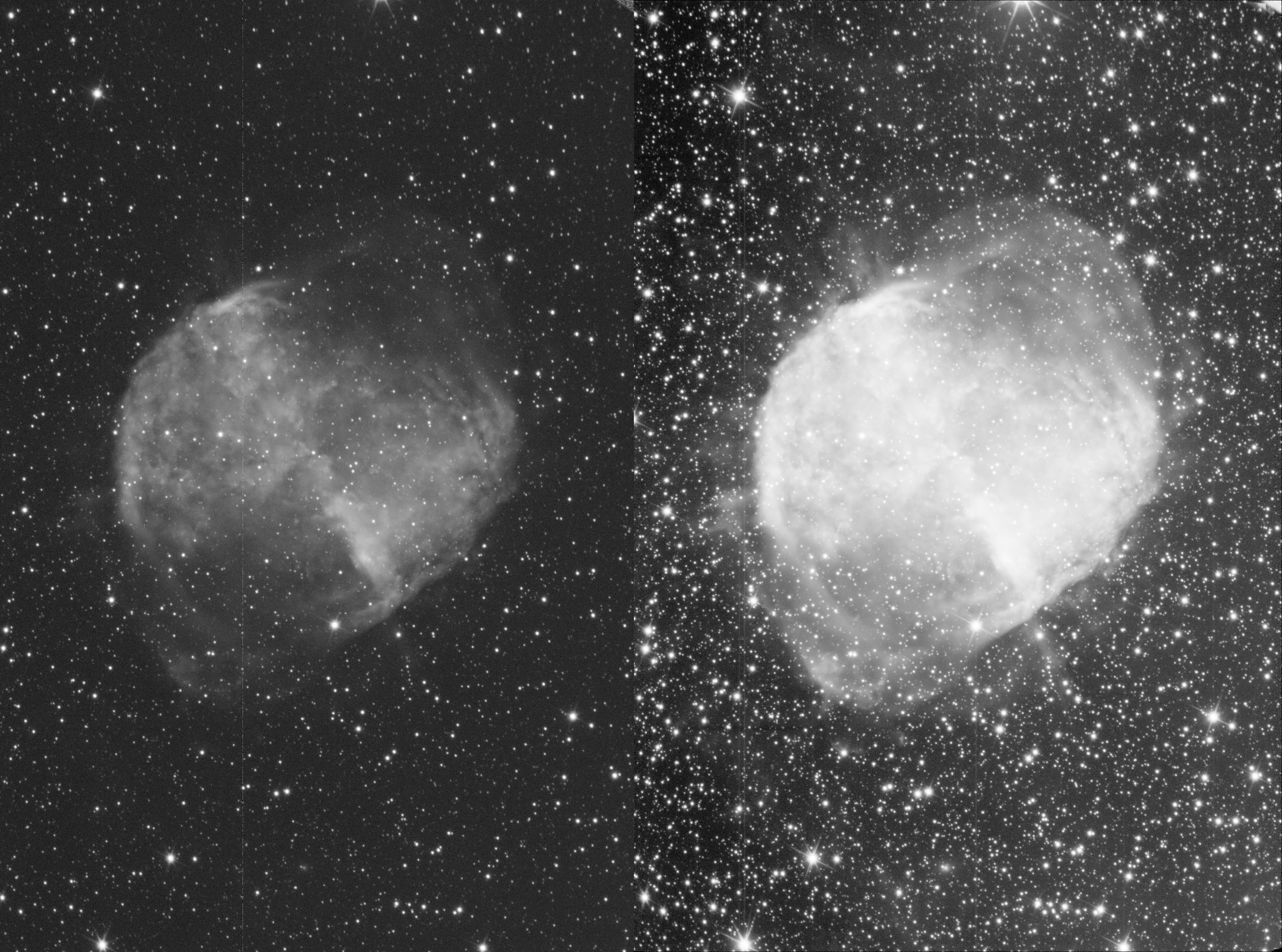
Here is the comparison of a single raw image and the integrated image for the R channel.
Work plan with integrated channels: find stars, shift and transform images together (in APP now unselect “same camera and optics”, and possibly select “use dynamic distortion correction”, plus if the number of stars in U is not very high, select the U channel to be the reference frame), save aligned channels one-by-one as fits files.
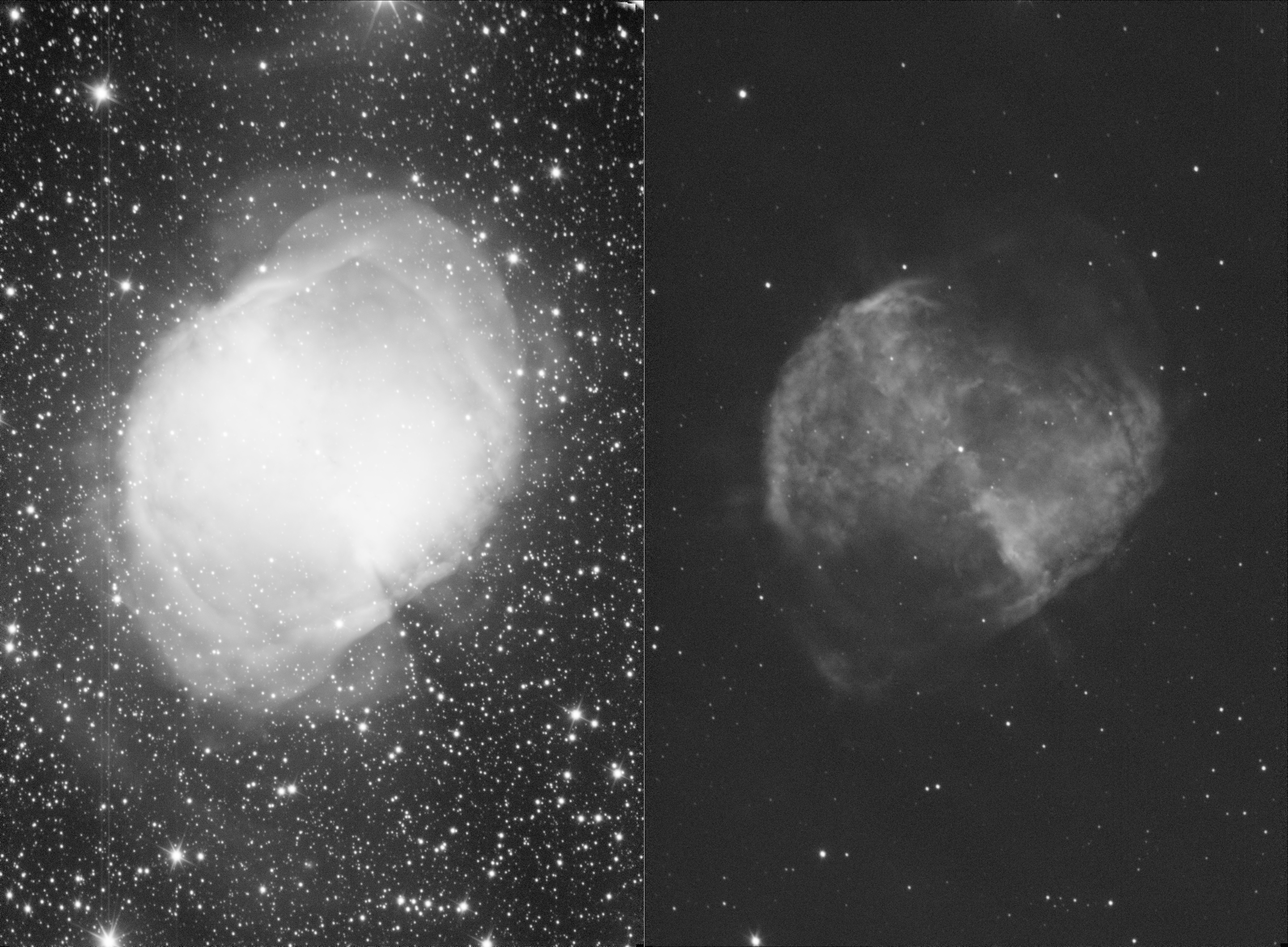
As an illustration, here are the two other integrated channels too (G and U).
Work plan with fully aligned integrated channels: in APP under “Tools” use the “Combine RGB” button to load in the three files that you saved in the previous step, set the R, G, and U channels to R, G, and B colours, and process to taste. You can play around with the curves, saturation and other settings later in other image processing applications too (e.g., Adobe Lightroom), for this, save the colour image from APP as a 16 bit TIFF file. If you used my python script for the reduction, flip your image vertically to get a true-to-sky orientation.
The rest of the photos I made with the MAIA camera can be seen after the click below (to save bandwidth), or towards the bottom of my flickr album.