1. Motivation
I am a professional astronomer who loves maps. But let me start with a small background story: I joined the Hungarian Astronomical Association in 1999 (the year of the great European total solar eclipse) at the age of 14, just after receiving a 76/700 Newton reflector from my parents for Christmas. Even though my love of astronomy dates back to long before that, joining the HAA was the start of my actual amateur astronomy career. I went on youth astronomy camps, where I tried to find as many Messier objects as I could under the dark rural skies of the Mátra mountains (besides regularly drawing sunspots and observing variable stars whenever I could), and for this I definitely needed a sky map.
Back then – just like 99% of the Hungarian amateurs – I had no money to order any of the nice star atlases from abroad (e.g., the actual edition of Uranometria 2000.0 was definitely high on my wish-list, but always way over my budget), so I used mostly the AAVSO charts for variable stars, and an “atlas” that I printed at home using a free version of the SkyMap Pro software. It took a few years until I managed to buy a proper atlas, thanks to the release of the “Égabrosz” in 2004, which was the first professional-quality sky atlas produced in Hungary. It was (and still is) a great black and white atlas positioned somewhere between Uranometria 2000.0 and Sky Atlas 2000.0 (based on its limited magnitude and resolution).
My practical participation in amateur astronomy ceased to continue soon after I started my university studies, and moving under the heavily light-polluted skies of Belgium did not help to reignite my interests later on, but I always kept my fascination towards mapping (the night sky), and I always wanted to make a proper (sky) atlas myself. Now that I know quite a lot about astronomical data, and I know how to make nice plots using the python programming language, I though the time was just about right to actually try and see if I can really make one. How difficult could it be, right?
2. Introduction
My goal was to produce a publication quality, both practical and visually pleasing star atlas aimed at amateur astronomers. To do this I had to first study the atlases currently available on the market, because I did not want to reinvent the wheel. Here is a non-complete list of the probably most widely-known atlases on the market:
While there are also a few free well-known atlases online:
Each atlas has their pros and cons. It is beyond the scope of this post to compare these atlases (but you find a nice comparison here, the text is in Polish, but the numbers and pictures are more important anyway), but there are a few things to consider when planning a new one. These are:
- Format (size, number of pages)
- Grayscale or colour
- Legibility (colours, font types, label placement, print quality)
- Resolution (scale in cm per degree of declination)
- Limiting magnitude (typically 7.5 – 11.5)
- Database and selection of non-stellar objects
- Representation of objects (marker shapes, sizes, etc.)
- Consistency (especially colour, line width, and font size)
I wanted to mix the best ingredients of these atlases, building around these main ideas:
- A layout similar to the one of Uranometria 2000.0
- Colours similar to Interstellarum Deep Sky Atlas
- Milky way contours similar to Sky Atlas 2000.0
And then add the following refinements / improvements into the mix:
- Slightly larger field of view (FOV) than in Uranometria 2000.0 with the full sky on 344 A4 – or alternatively B4 – pages (1.6 cm per degree or 1.9 cm per degree)
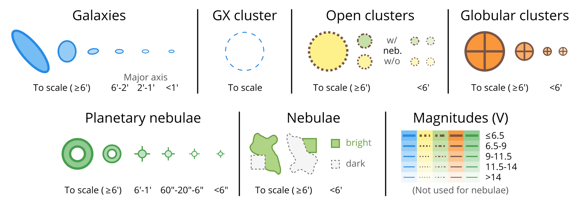
- Non-stellar objects are printed to scale (down to a cutoff size), line width and fill colour relating to the actual brightness
- Legible colour scheme: avoid using red since it is invisible under red light
- Precise Milky Way representation (unlike in any printed atlas)
- Clever navigation between pages
- Hand-drawn bright and dark nebula outlines from scratch
- Nice custom typography
- Vector graphics
- Automated label placement
- Automated compilation of the full atlas by a press of the button
- Flexible script (change FOV, magnitude limit, colours with ease)
I will go over all these aspects in detail in the following section and explain step-by-step how I built the atlas. As it is not 100% done yet, I will also note down the features that still need to be completed or refined in the (hopefully) near future. I started working on this during the first days of March, and by the middle of April most of the things that I am going to discuss here were done. Since then I spent less time on the project and took care of minor refinements only.
3. Practical execution – techniques and design aspects
3.1 Python setup
I am using a very basic setup installed via Canopy. My main environment is python 2.7, and I make use of the following packages extensively:
- numpy for all kinds of data handling and numerical operations
- pylab / matplotlib for all the main plotting operations
- basemap for the mapping (takes care of the projection and the related transformations)
- scipy for some specific interpolations and contours connected to the Milky Way
- astropy and pyephem for celestial coordinate transformations
3.2 Source data
All databases that I am using are either publicly available from the internet (under various licences), or they are compiled by me from publicly available data (which is discussed in the following sections).
- I/259 The Tycho-2 Catalogue (Hog+ 2000) [Main catalog + Supplement 1]:
stars with position, magnitude, proper motion, and multiplicity information
- B/gcvs General Catalogue of Variable Stars (Samus+ 2007-2013):
variable stars’ name, type, minimum, and maximum brightness information
- V/50 Bright Star Catalogue, 5th Revised Ed. (Hoffleit+, 1991):
Bayer and/or Flamsteed name(s) of bright stars
- IAU Catalog of Star Names (IAU-CSN):
common star names approved by the IAU (not yet implemented, but already prepared)
- Saguaro Astronomy Club Database version 8.1:
database of deep sky objects
- VI/49 Constellation Boundary Data (Davenhall+ 1989):
IAU constellation border data, overlapping (duplicate) border lines removed by Pierre Barbier
- Constellation lines’ data:
currently a data file from KStars
in the future I will implement the figures that are shown at the site of the IAU*
*there are no official constellation figures, only the boundaries are set in stone by the IAU
3.3 Custom, and compiled / processed databases
While some of the data can be used as is (for example the data of constellation boundaries and lines), most data needs to be first processed in a way or another before it is ready to be plotted. There are three large groups that need to be dealt with: stellar data, milky way contour data, and deep sky data (with a large stress on extended bright and dark nebulae).
3.3.1 Stellar database
Building the stellar database is taken care of inside the main plotting script (which will be discussed in detail in Section 3.4). Every time the script is executed, it checks if a precompiled magnitude limited stellar database is already available, and if not, it builds it from the databases discussed in Section 3.2. When the script is ran with a given magnitude limit for the first time, a new magnitude limited database must to be compiled, which happens in multiple stages (and at a magnitude limit of 10.0 it takes ~3 hours to complete):
- Tycho-2 data read in and magnitude limit applied (after computing V magnitudes from the available BT and VT magnitudes), magnitude limited Tycho-2 data saved.
- Bright Star Catalog (BSC) data read in, magnitude limit applied, names formatted to a pylab / LaTeX compatible format (so when annotating later on, proper Greek characters will appear automatically), magnitude limited BSC data saved.
- General Catalogue of Variable Stars (GCVS) data read in, stars in maximum dimmer than the magnitude limit thrown out, stars with an amplitude less than 0.1 mag (rounded to 1 decimal) are thrown away, and stars of some selected types such as Novae and Supernovae are thrown out, names formatted, then the remaining data is filtered and formatted, magnitude limited GCVS data is saved.
- The filtered GCVS data is used to update the filtered Tycho-2 data. First the GCVS coordinates are cross-matched one-by-one with the Tycho-2 coordinates (within 6″). There are three possible outcomes of this match:
a) there are multiple Tycho-2 stars within 6″ from the coordinates of a given GCVS star (which happens sometimes in crowded areas), then we use the maximum magnitude information to match the Tycho-2 magnitudes, and update the best matching Tycho-2 entry with minimum and maximum magnitudes, the GCVS name, and a variability flag = 1
b) there is only one match (which is the most common case), when life is easy, the GCVS entry is for that Tycho-2 star, so we add the magnitudes, the variable name, and the variability flag = 1 to the Tycho-2 entry
c) there is no match (a rare case, but happens, e.g. when an irregular variable was much dimmer during the Hipparcos measurements then the magnitude limit, but on a longer period it can get brighter), then we need to add the GCVS star as it is to the compiled catalog, because it is not yet in the magnitude limited Tycho-2 sample.
After this is done, the magnitude limited database with variability information is saved, and later on in the plotting stage stars with a variability flag = 1 will be plotted with a spacial symbol.
- In the next step, this database is updated with multiplicity information (in our case a multiplicity flag, and a separation value for the two brightest components). The reason for this is that for stars that appear closer to each other than a threshold (in our case this is set to be 60″), we do not want to plot each component, only the brightest one with a special symbol, which is common practice in stellar atlases. (Small not here: at this point, components that are closer to each other than 0.8″ are not included, but resolving stars that are so narrowly separated is practically impossible visually and/or without professional telescopes and exceptional weather conditions.) This is also done in multiple steps:
a) stars are ordered from brightest to dimmest, each given a multiplicity flag = 0 to start with
b) starting from the brightest we check each star one-by-one if there are other (dimmer) stars within 60″ from it
c) if yes, then the brightest component (A) gets a multiplicity flag = 1 and the dimmer component(s) (B,…) get(s) a multiplicity flag = -1
d) in the next steps only stars with multiplicity flag != -1 are tested as potential components, which means that, e.g., we will not identify a dimmer star later on as primary component when it was already found to be a secondary component of a brighter star earlier
e) later on in the plotting stage only those stars will be plotted where the multiplicity flag is not -1, and from these the stars where the multiplicity flag = 1 will be plotted using a special symbol.
When this is done, the data file is saved (now containing a magnitude limited Tycho-2 database that is updated with variability and multiplicity information). This step takes the longest time of all by a significant margin.
- In the last step this database is updated with names from the precompiled magnitude limited BSC file that was saved in step 2, similarly to how the GCVS entries were matched in step 4, but with a slightly higher tolerance in the coordinate match (to adjust for the possible apparent merging of multiple stars’ coordinates in step 5). Then this database is saved as the final stellar database of the atlas.
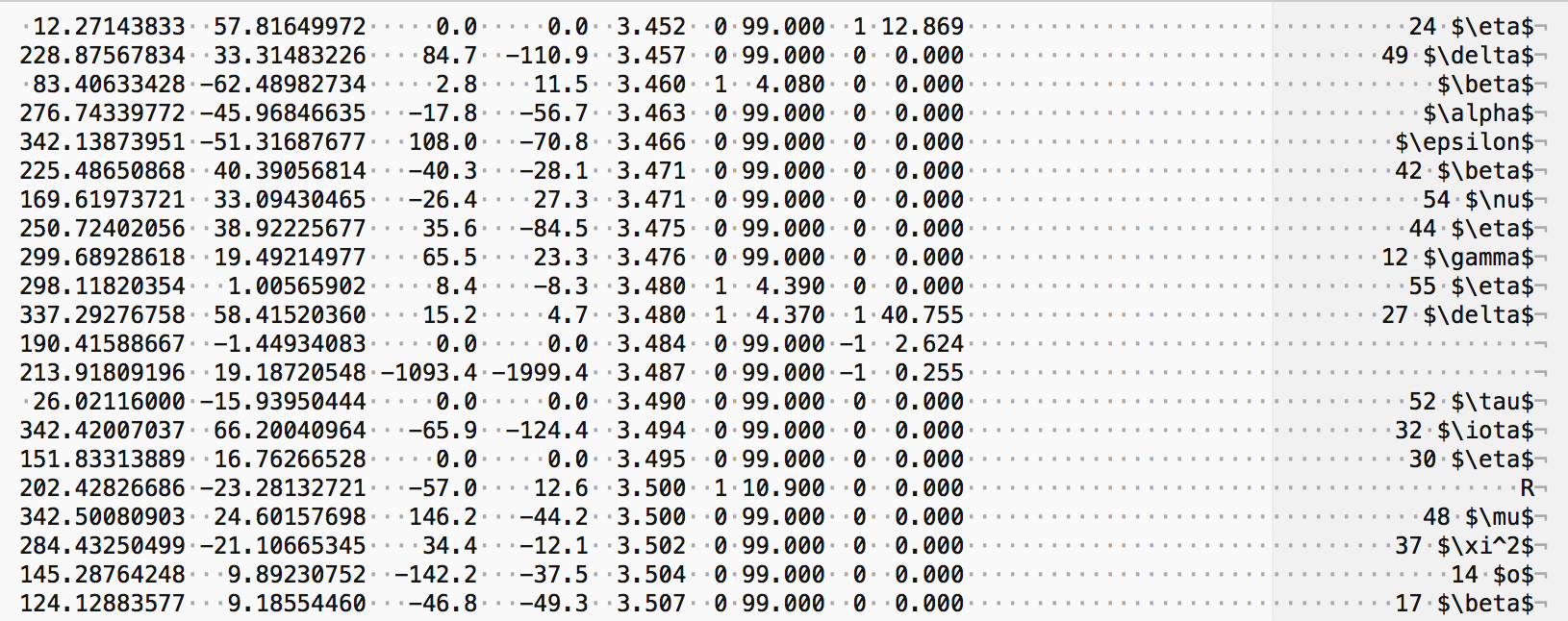
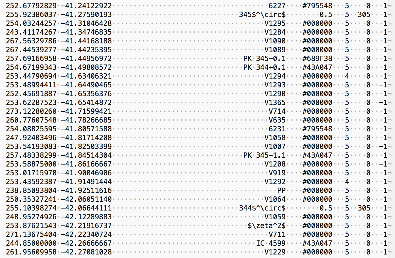
At this stage here is how a small section of the compiled stellar database looks like with a pair of coordinates, a pair of proper motions, a visual magnitude (which is a maximum brightness for variables), a variability flag, a possible minimum brightness (set to 99.000 for non variable stars), a multiplicity flag, a separation value of the brightest components for stars that have a multiplicity flag of 1 (otherwise set to 0.000), and a name (excluding the abbreviation of the constellation) in LaTeX format:
3.3.2 Contours of the Milky Way
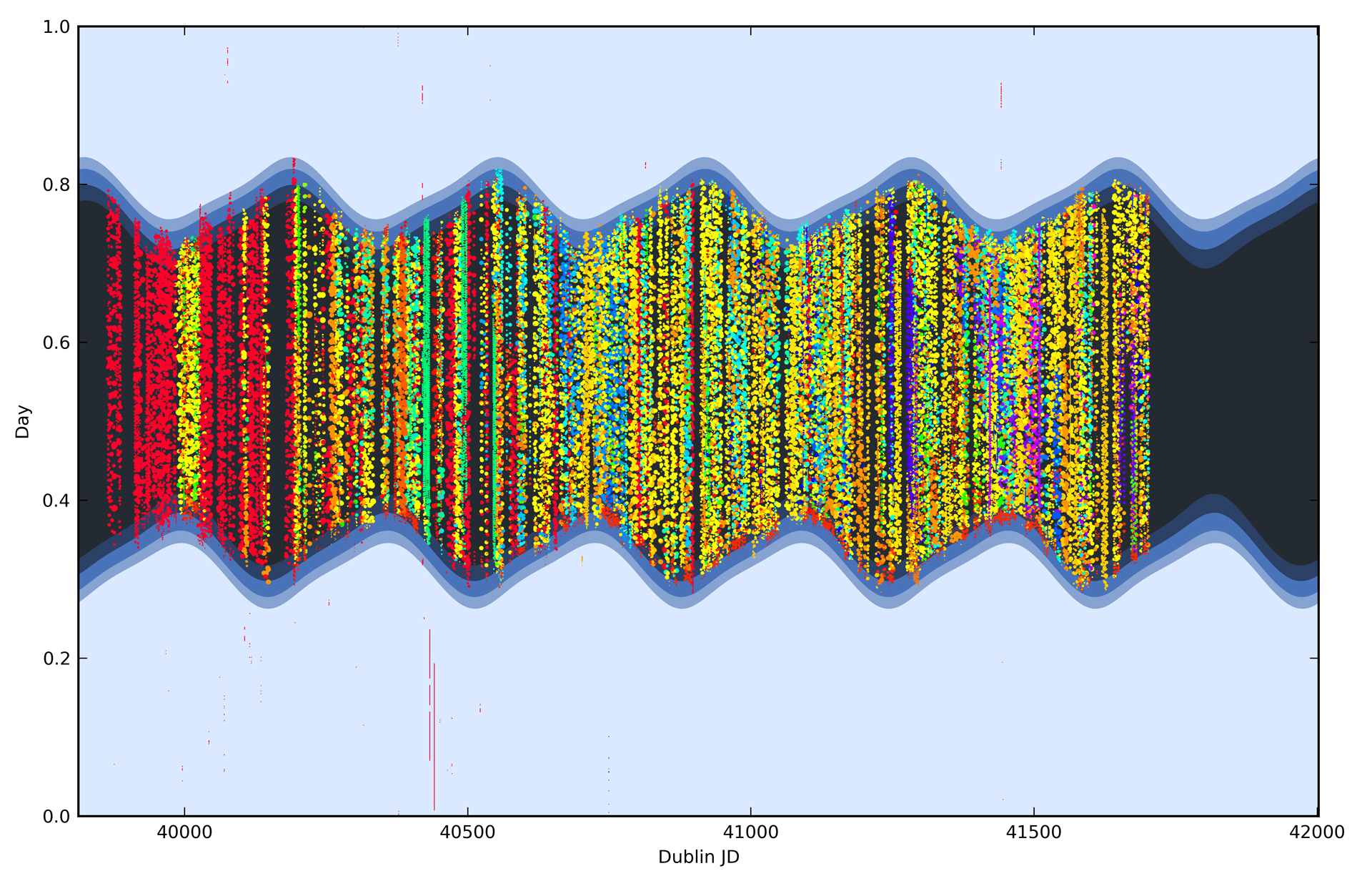
One of the main new features of my atlas (compared to other atlases on the market) is the inclusion of the (as) precise (as possible) contours of the Milky Way on its pages. For this I had to make my own data. I started from the APOD of the Milky Way by Nick Risinger (for which I still need to ask permission if I want to get this atlas distributed). I scaled this up slightly to 3600×1800 pixels (to match the 360×180 degree size of the full sky with a 0.1 degree pixel size), converted it to grayscale, applied a star-removal filter, a small blur, and enhanced the contrast slightly. Then using python I converted it to an array of brightness data on the galactic coordinate grid, and after a coordinate transformation from the galactic to the equatorial frame I saved it in a numpy specific file format using the numpy.savez() function.
This specific format is needed because reading in a 150 MB ASCII file is too slow with numpy, and it would create a bottleneck in speed when plotting the atlas pages. I use this brightness data later during the plotting and display it using contours set at some cleverly specified brightness levels to create a both visually pleasing and highly-realistic image of the Milky Way. The results are very nice, e.g., one can see multiple brightness levels even inside the Magellanic Clouds (as it can be seen below, but for the sake of clarity plotted using stronger colours than what is actually used in the atlas).
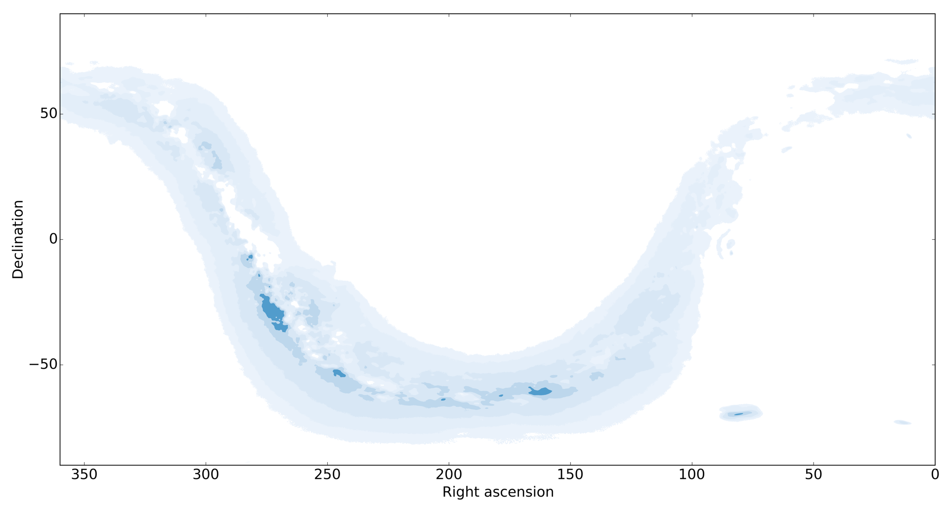
I also tested if the coordinates of the original image were correct by repeating the same steps but without removing the stars, so one could actually see the stars on the contour plot too. In this experiment they lined up perfectly with the actual stellar data, confirming that the position data in the Milky Way image was correct.
3.3.3 Deep sky objects (contours of extended bright and dark nebulae)
The SAC database is a good starting point, since it has a great selection of objects that are accessible with a various range if amateur instruments. On the other hand, it has quite a few mistakes too, so I had to work on it a bit to make it more consistent and less messy. First of all I checked all objects that have an apparent size larger than 12′ (twice the cutoff size of my atlas) manually in DSS using the Aladin desktop client, and corrected sizes and/or position angles where I found it necessary (only a few cases). I also removed all duplicate entries from the database (which occurred with quite a few galaxies: many had multiple entries from different catalogues). I also decided to filter out those objects that had no useful/trustworthy brightness information (dropping mostly small open clusters that were barely identifiable on the DSS images anyway), and those open clusters that appeared too large on the scale of the atlas (typically the ones above 100′-120′, depending on the density of the field). Finally, I made sure that for Messier objects the Messier entry is used as name later on, not the NGC one. These were the easier parts.
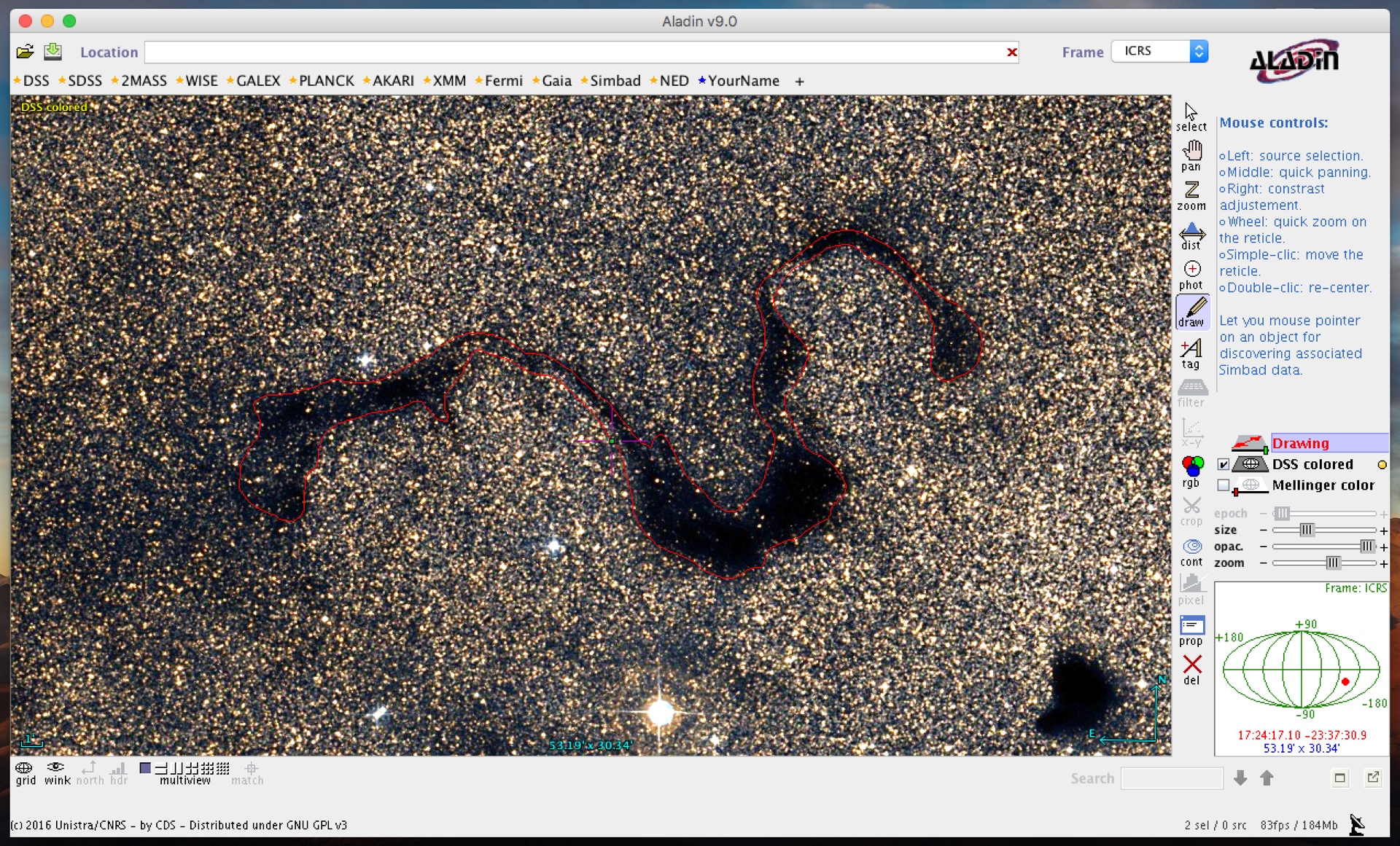
The more difficult and time consuming part (taking around 40-50 hours) was drawing all bright and dark nebulae from the SAC database larger than 6′-12′ (meaning that 100% of the objects that are at 12′ or larger in diameter had to be drawn, and some of the smaller non-symmetric ones too), which I had to do manually, along with a few missing ones that I found worthy by looking through images in Aladin or by cross-checking with the selection on Sky Atlas 2000.0’s pages. (I am aware that there is a set of nebula outlines available online by Mark Smedley and Jan Kotek, but I did not find these good enough for my needs, and I did not want to copy other people’s data to begin with, because nebula outlines are one of those elements of an atlas that make it personal.) In practice I used Aladin to draw the contours of these objects with a mouse (I wish sometimes that I had a proper tablet and a digital pencil to do such things…), and export them as coordinate arrays.
For the brighter ones I tried to make the contours resemble the visual look based on drawings done by amateurs, while for the more difficult targets I went with the expected photographic outlines. It helped a lot that Aladin can create contour plots on the displayed images, leading my eyes while tracking the outlines. (For this I used the Mellinger Optical Survey and the DSS layers.) Some complex or large nebulae are drawn in multiple sections, for example the Vela Supernova Remnant in 22 pieces, IC 1318 in 14 pieces, and Sh2-240 in 42 pieces. Here is a rough example how this process looks like in Aladin:
3.4 Plotting one page of the atlas
There is one single python script that takes care of the plotting of a single page of the atlas (plot_map.py). At the moment it is 1545 lines long, and contains – among others – 16 custom functions (some of which will be discussed later).
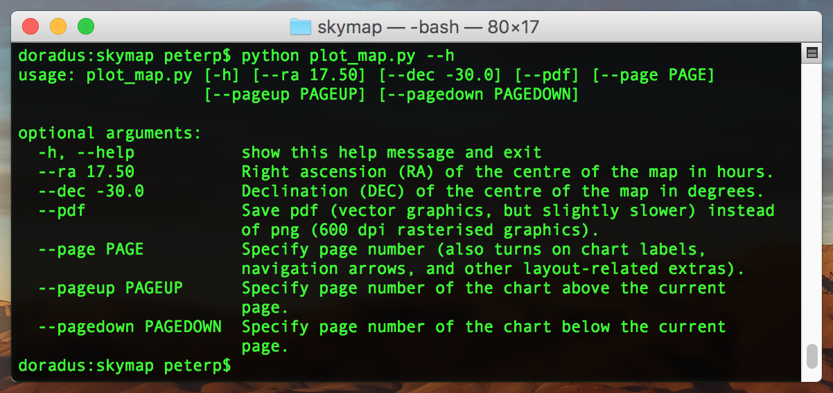
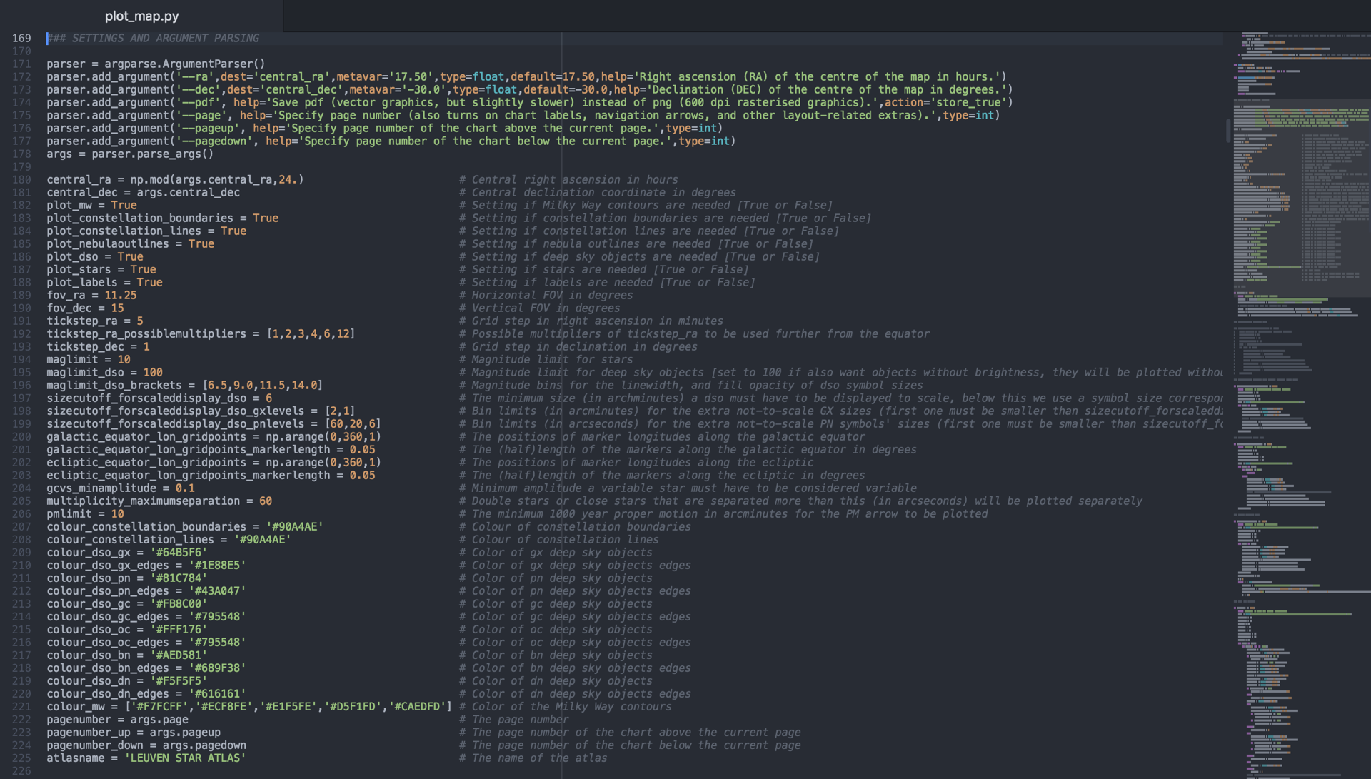
3.4.1 Arguments and control variables
To control what and how is plotted by the script, I am using a small set of arguments, and a larger set of variables (that I like to call control variables). These are separate for a good reason. Arguments can be given (values) simply from the terminal when running the script, and as such they can be also set by a higher level python script when compiling the whole atlas (see Section 3.5). These set the centre of the field of view, the output format (vector – pdf, or raster – png), and optionally the page number along with the page numbers of the pages that show the field above and below (thus up and down in declination) the current page in the atlas. These last three are optional, and when not given the script will simply produce a sky chart without the extra formatting of an atlas page.
On the other hand control variables have to be set inside the main script, and they control the colours, size and magnitude limits, the different types of objects that need to be plotted, the field of view, etc. These stay the same for each page.
Later on when closeup charts and chart index pages are created I will save a different version for each (e.g., plot_map_closeup.py and plot_map_index.py), where the limited magnitude, and a few other things will be set differently.
3.4.2 Colours and typography
When choosing the colours I experimented a bit with different colour combinations, but the main principles were always the same. I had to avoid red because it is invisible when the chart is browsed using a red torch (and this is common practice, since red light interferes the least with our dark-adapted eyes), and I wanted colours that go well together, but are easy to distinguish. At the end I choose my palette from Google’s material design guide.
When choosing the individual colours, the following ideas were factored into my decisions. First of all, I wanted the Milky Way to be plotted as shades of blue, not only because that looks great in Sky Atlas 2000.0, but also because the most prominent structures in a galaxy – the spiral arms – consist of young massive stars, and they are predominantly blueish in colour. As a consequence all galaxies had to be plotted in blue. Groups of stars are yellow as in most other colour atlases, but globular clusters are orange, since these are dominated by old(er), low-mass stars, and thus their light (spectrum) is more shifted towards this colour. Planetary nebulae are green, because the strongest emission line in their spectrum in the range where our eyes are the most sensitive is the [OIII] line at 500.7 nm, which appears to be green. Even though other types of bright nebulae might have different spectra (especially bright reflection nebulae), they are also plotted green (although a slightly different hue) to stay consistent. Stars are black and map-related lines are different shades of grey.
Outlines are always darker than the fill colours, and while the outline colours are constant, the line width and the opacity of the fill depend on the magnitude of a given object. Labels are always the same colour as the labelled objects’ outline.
I am using the Open Sans font family throughout the atlas, this is a nice, free, slightly narrower than default sans serif font with an extensive set of glyphs (including all necessary accented and Greek characters), that provides excellent legibility in many font sizes and weights (of which I am using the regular and bold variants).
3.4.3 Vertical layering
One important thing to handle when printing the chart is the vertical layering (or hierarchy) of the different object types, but also the vertical layering within a given object type. This way we can avoid larger objects overlapping – and blocking from view – smaller ones. Therefore, for example, the Milky Way needs to be plotted under everything else, dark nebulae need to be plotted over bright nebulae, small galaxies need to be plotted over large galaxies (otherwise, e.g, M 32 in the Andromeda Galaxy would not even be visible), stars need to be plotted over deep sky objects (so they are not covered by extended objects), and dim stars need to be plotted over bright stars (otherwise some dim stars close to bright stars could be covered by the larger disk of the bright star).
Placing different object types on different vertical layers is taken care using the zorder keyword inside any king of plotting command in python, while the required hierarchy within a given object type is ensured by sorting the objects according to size (from large to small, or from bright do dim in the case of stars), which means that when they are plotted by a plotting routine later on, they will be plotted according to the order they were sorted into. There are some special cases where the plotting order of open clusters and bright nebulae needs to be flipped (where a larger open cluster includes a smaller bright nebula), but this is also taken care of with a zorder-modifier value in the database of the hand-drawn nebulae, which effectively moves the given nebula to a layer above the open cluster.
3.4.4 Setting up the page
Before plotting any celestial data, we need to set up the plotting environment to be able to work with celestial coordinates. As already mentioned before, I use the basemap library to do this:
map = Basemap(projection=’stere’, width=fov_ra, height=fov_dec, lat_ts=central_dec, lat_0=central_dec, lon_0=360-(central_ra*15), celestial=True, rsphere=180/math.pi)
By using the celestial=True setting we make sure that we use the astronomical conventions for longitude (negative longitudes to the East of zero), and by setting the radius of the sphere to be 180/pi we can give the horizontal and vertical size of the area covered in the projection in degrees.
Like most celestial atlases I also use the stereographic projection. This is a conformal projection, meaning that it preserves the angles, but it does not preserve distances or areas. (There is no projection which would preserve all of these.) While indeed towards the edges equal distances seem to get larger, this effect is practically negligible at zoom levels that are used in a celestial atlas like this one.
After the map environment is set, we need to draw the grid of latitude and longitude lines (using the ICRS frame and a standard J2000.0 epoch), and I make sure that none of these lines get too dense as we get close to the poles, by tapering selected meridian lines before they reach the poles (see below). The density of the labelled meridian lines is also set by the distance from the pole, so labels never get too dense around the edges of the map area.
After the celestial grid is set up, I draw the ecliptic and the galactic equator along with the ecliptic and galactic poles, and small tick markers for each degree along the equator lines. Drawing the equators is very easy, one just needs to transform a constant (ecliptic or galactic) latitude = 0° line from ecliptic or galactic coordinates to equatorial coordinates, and plot the resulting array as a line. When drawing the poles, I draw their X shaped markers from two separate perpendicular lines (crossing at the poles) which point towards longitudes 0°, 90°, 180°, and 270°, this way, e.g., when looking at the galactic poles the reader can see how the galactic coordinate frame is rotated very differently compared to the equatorial grid.
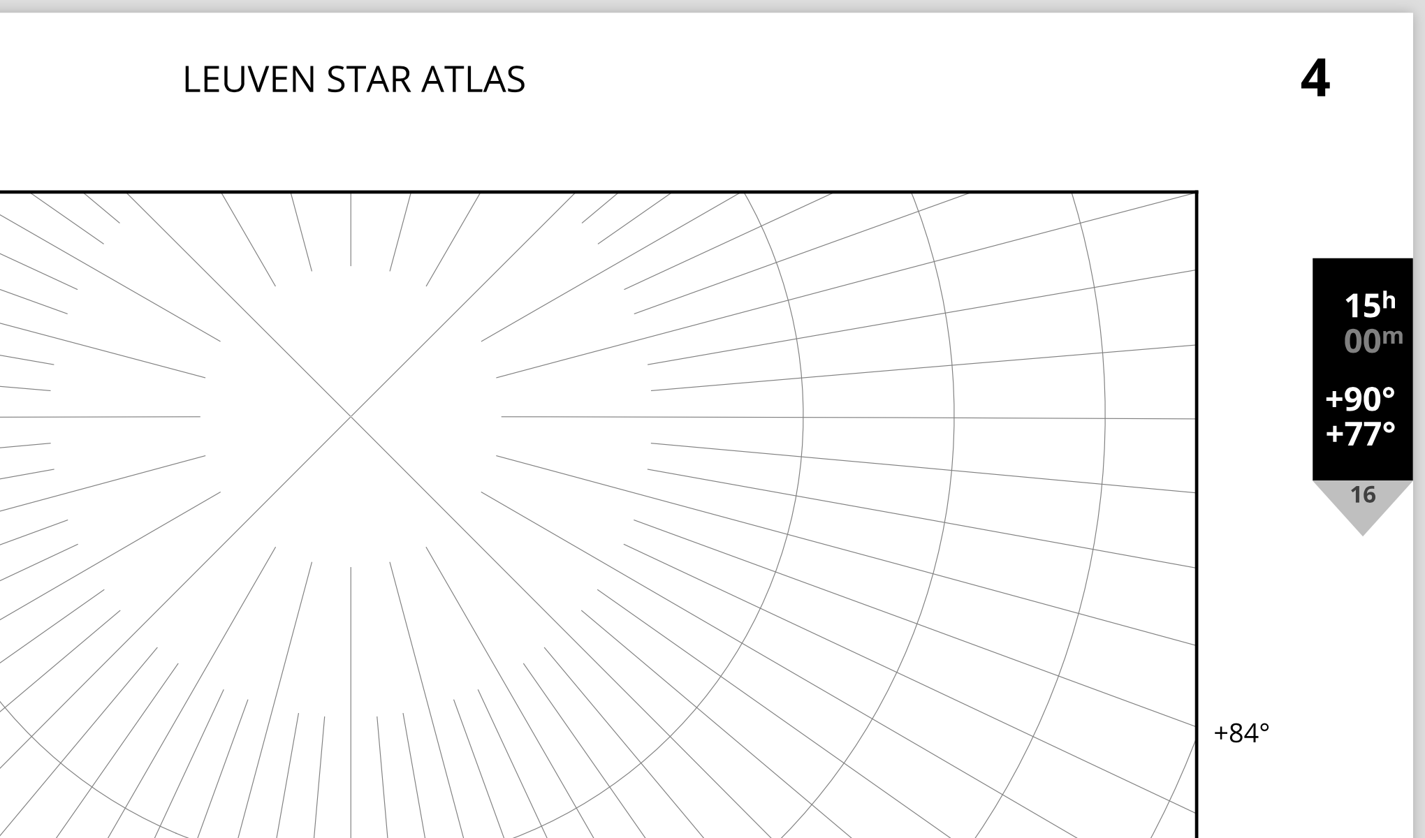
As we are trying to produce not only a simple sky chart but a page in a stellar atlas, we also need to plot page numbers, navigation aids, and a legend box. Page numbers are plotted in the top and bottom outside corners (from a double page point of view) , which makes it easy to flip through the atlas when looking for a page number. There is also a special navigation bar plotted along the outer edge of each page. This navigation bar shows the central RA coordinate of the page, the minimum and maximum declination values of the page, and also the page number(s) of the closest neighbouring page(s) in declination (a.k.a. the pages above and below the current field). The location of this feature along the edge of the page depends on the central declination of the page. This means that just by looking at the edge of the closed atlas, or while flipping through it, the user can immediately see which region of the sky they are heading towards from the position of the navigation bar. (For example, on a page towards the North Celestial Pole this bar will be near the top of the edge of the page, while for pages around the Celestial Equator it will be at its centre.)
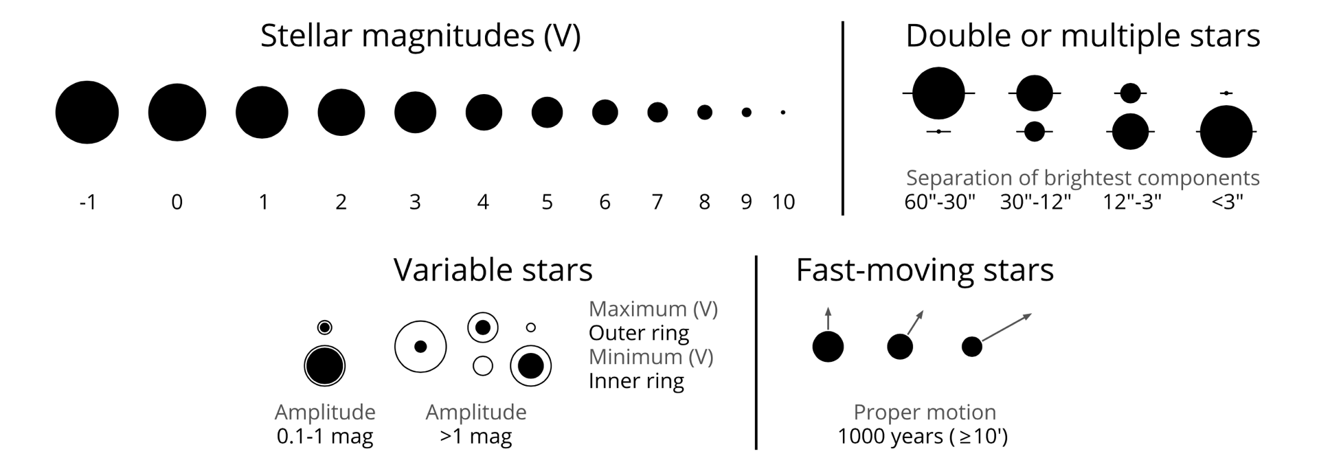
Creating the legend box gave birth to probably the most interesting solution (in terms of coding) in the production of the atlas. In the following sections I will show that I set the size of all objects on the map using angles (angular diameters), and not by using marker sizes (in points or pixels) as done by default in python. This is very useful in the main map area of the page, but it meant that I had no idea how large an actual marker was when not working in a map instance. Therefore I could not simply create a simple subplot below the main map area and place the different symbols and their keys there without writing transformation functions to make sure that the size scales between the legend area and the main map area match. Instead of this, I created a 1 degree tall subplot with the same basemap settings (so also the same width in degrees, resulting in the same scale) as the main map area above, meaning that I could use the same functions and scales to plot objects here as I do in the main plot. Creating the legends themselves afterwards was only a question of placing a set of given objects next to each other, making sure that they are properly spaced, and that their labels are at the same horizontal levels. Odd and even pages got different legend boxes, so a double page always shows a full set of legends (stellar objects and lines on the left hand page, and deep sky objects on the right hand side – see examples later on).
I do not want to discuss all the remaining details here, but every piece of text (e.g., page numbers, the numbers in the navigation box, etc.) is aligned with other lines or texts in a very strict way to ensure symmetry at all times, no matter what area of the sky is being plotted. There was a very large effort put into this, even though the reader might not (consciously) notice these fine details.
3.4.5 Plotting stellar data
I have written one single function to handle the plotting of stars, from the simplest single stars to multiple variable systems with high proper motions:
draw_screen_star(ra, dec, pm_ra, pm_dec, pmlimit, mag, maglimit, map, double=0, sep=0, variable=0, vmin=0, facecolor=’k’, edgecolor=’w’, zorder=90)
Stars are plotted from bright to dim as mentioned earlier. All plotting is done in map (sky) coordinates, meaning that the symbol sizes are given in degrees, and there is an inverse linear scale between symbol radius and magnitude value. All stars are plotted with a white edge, so if symbols of nearby stars overlap, they remain nicely visible.
The width of this wide edge is set to be the narrowest well visible line width in print (matching the width of the lines of the celestial grid), while the smallest stars’ size is set by the symbol of the dimmest variable star (where the black central region needs another white filling, which must be still well visible). The size of the largest star is set to be aesthetically pleasing (not too small so bright stars can be well differentiated from dim ones, but not too large so they do not became overly extended). This also sets the other fix point of the linear magnitude scale. On the figure below you can see various tests of the star plotting function, with one notable example of a set of stars plotted on top of each other where the magnitudes range from -2 to 10 with a step size of 1 (resulting in a nice well separated pattern).
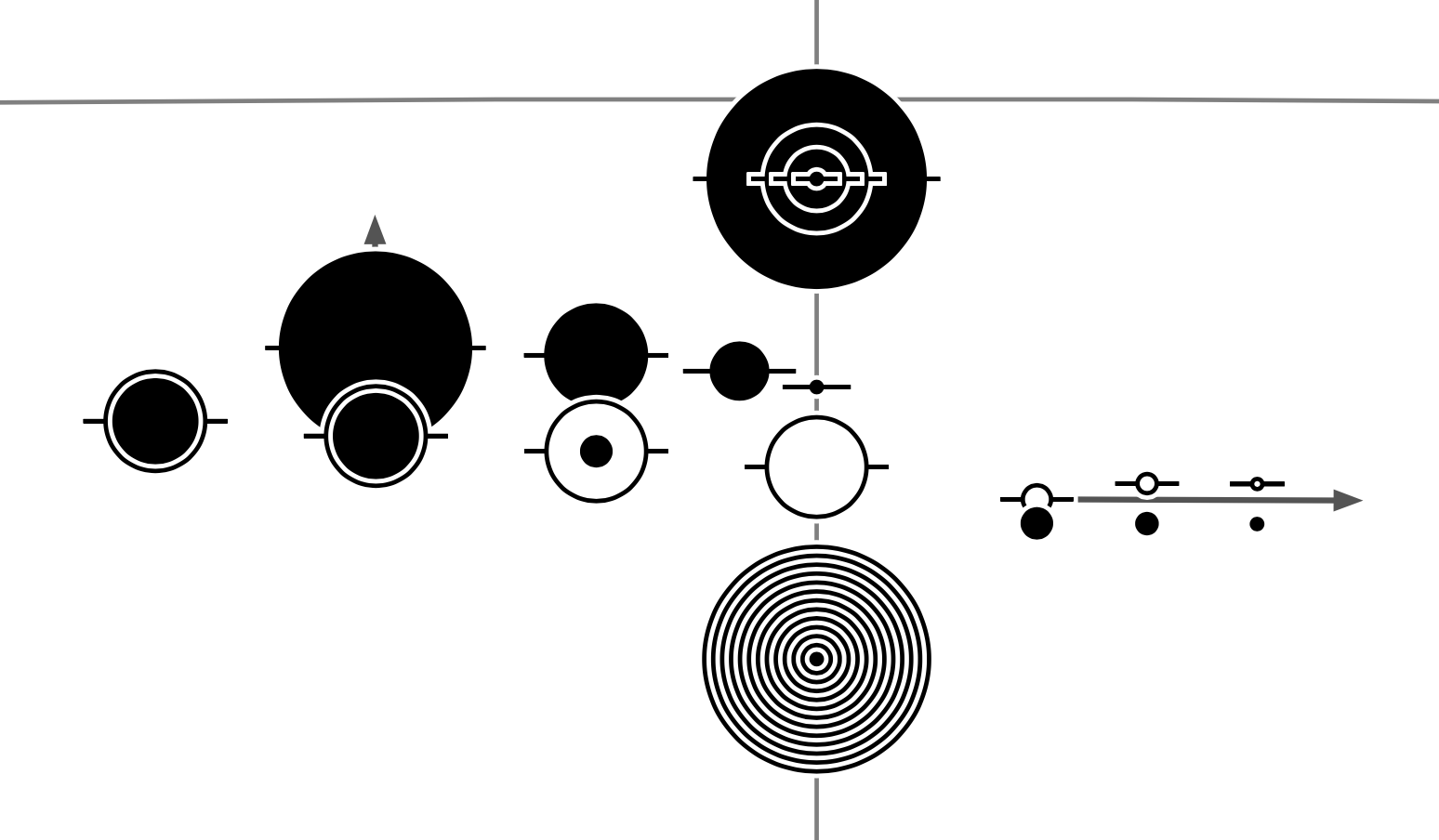
In practice, taking the example of a variable double star (where the star is also visible in minimum, so, e.g., the 3rd star from the left in the row of multiple variable stars), this is how the star symbol is created: first a white circle is plotted and a white bar across (these will be the white outlines), then a narrower black line (corresponding to the separation of the brightest components of the multiple system) and a black circle with a smaller radius (corresponding to the brightness of the variable star in maximum), followed by another white circle with a smaller radius (the inner fill of the variable), and finally a smaller black circle (with a radius corresponding to the minimum brightness of the star). If the star has a high proper motion, it is also plotted with an arrow in the background. In summary, the symbol of a star is built from a set of pylab.patches (circles, polygons, and fancyarrows).
Not strictly speaking stellar data, but I note here that constellation boundaries and stick figures are also plotted using simple lines. It is worth noting that to avoid plotting the overlapping sections of neighbouring constellations’ borders twice (which could introduce artefacts in the representation of dashed lines), I am using a version of this data where the duplicate line sections were removed.
3.4.6 Plotting non-stellar data
Similar to the stars, all deep sky objects are plotted in sky coordinates using specific functions that I have written for each different object type so I can feed sizes in arc minutes into them. The symbols are again made from various pylab.patches (ellipses, wedges, and rectangles) inside these functions. As an example, the symbol of global clusters is made out of four wedges that have a 90° opening angle (instead of trying to draw a nice cross inside a circle, which believe me is not as easy as it sounds). But outside of the function drawing a GC looks simply like this:
draw_screen_gcsymbol(ra, dec, size ,map, **kwargs)
Objects are plotted to scale when larger than a cutoff size (6′ in the LSA), otherwise they are plotted at given (smaller) fix sizes depending on which size-bin they fall inside the category. As mentioned earlier, the edge line width and the fill colour represents the visual brightness of a given object. The orientation (position angle, or PA) of galaxies is plotted true to reality, and to do this the local North had to be calculated at each position in the map (with a small function), which was then used to correct the PA coming from the SAC catalog (since on our map North is only ‘up’ along the central longitude of each page – except for right above the North and right below the South Celestial Poles, where the apparent direction of North along the central meridian is inverted).
I have kept most of the classical symbols, with the exception that planetary nebulae that are larger than the cutoff size (so planetary nebula that are plotted to scale) are plotted with a doughnut symbol (symbolising the classical PN look). Size bins were chosen so they are more or less equally populated by the smaller objects.
3.4.7 Labelling objects
The last large task in creating a page in the atlas is labelling all plotted objects. My original goal was a fully automated setup based on the adjustText package, but this seems to be a much larger challenge to implement than first thought. The package works relatively well when labelling a set of small points or a set of objects that have the same size, but things get complicated when one wants to label a mix of patch objects (that have various sizes) and lines… Therefore after some experimenting I decided to put the automatisation attempts aside, and write a labelling graphical user interface (GUI). In any case even if the automated labelling would work, I would need this GUI to be able to make refinements in the label placements.
The main idea is that I run a slightly modified version of the original plot_map.py script (label_map.py, updated with the functions that make up the GUI), which produces an interactive version of the given page where I can just click on the labels (that are placed at the bottom right corner of each object by default as a starting point) and manipulate them. Using the GUI I can move labels (this way I can place them in a way that there is no overlap between objects and labels), I can make labels disappear (should a region be too busy for all labels to be visible), and I can even add in additional labels (to label the constellations, the poles, and the Magellanic Clouds – since they are plotted using the Milky Way contours and not as separate objects with their own label entries). When the GUI is run for the first time, all plotted objects are also fed into the
appendtolabellist(ra, dec, name, colour, size, rotation=0, visibility=1)
function, which builds a label table (from the names that were already available both in the stellar database and in the deep sky database) for the given page (placement positions, label texts, sizes, colours, rotation values – that are used for the labels of the ecliptic and galactic equator -, and a visibility flag), that I can modify with the GUI, and export it to be used by the main plot_map.py script. See part of such a label table below for a dense Southern part of Scorpion.
If the label table is available for a given page when the plot_map.py script is used, labels will be also plotted. The advantage of having an actual label table (so a file like labels_P_004.txt for Page 4) for each page is that I can also modify label texts and sizes manually to fine-tune details for the final version, without having to edit the original object databases.
Of course since now I have to move almost all labels around manually, it takes a while to make the label table for a page (even with a good default offset from the corresponding symbol, there are so many stars that the chance that the default placement will overlap with something is pretty big). In practice this can be anything from ~20 minutes to 2 hours depending on how dense the filed is… My estimate is that labelling all pages would easily require 300 hours of work. Or I need to come up with a clever solution and write an advanced function to move the labels around automatically, but this seems equally difficult to me right now. So for the time being I labelled 5 sample pages that can be seen in Section 4, and depending on the future distribution of the atlas (proper printed version or only on-line for free), I will see how much effort and what kind of effort I need/want to put into labelling the rest.
The animation below shows how the formatting and the different layers of objects come together to form one page of the atlas.
3.5 Plotting the whole atlas in one go
Plotting the whole atlas is taken care by a separate script called plot_atlas.py: this is only 91 lines long, and has a very limited amount of tasks to do. First of all it has a list of the central coordinates of the atlas pages (given as an equidistant list of declinations, and for each declination a list of right ascensions).
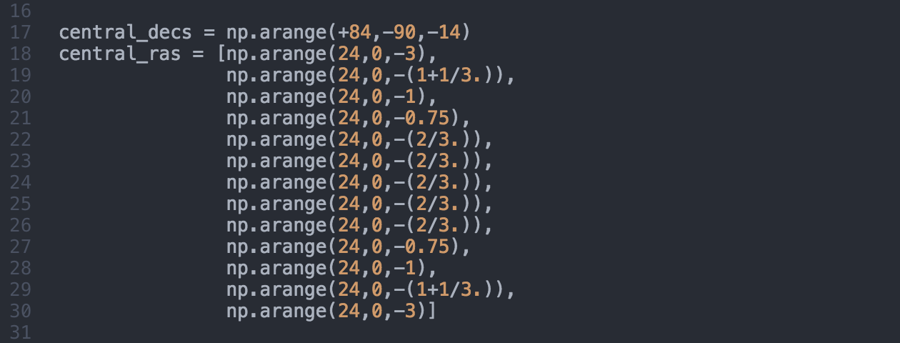
From this the script compiles the set of arguments that were discussed in Section 3.4.1 for each page by first building a list of page numbers and central coordinates, then calculating the closest (neighbouring) pages in declination (to North and South) for each page, which are stored as the pageup and pagedown values, respectively. Finally the script simply calls the plot_map.py script for each page – feeding the corresponding list of arguments to it – to initiate their production one-by-one (or four-by-four when using all available cores).
The whole process takes around 4 hours on my laptop (using 4 cores in parallel). This time could actually be still shortened quite significantly, because right now all data files (e.g., the magnitude limited stellar catalog, or the deep sky catalog) are read in for each page over and over again, instead of just keeping them in the memory after the first read in operation. This originates from the fact that the plot_map.py script is written as a standalone script that can produce a page of a stellar atlas or a simple star map from scratch (and even compile databases from existing databases as we have seen it earlier) if necessary, and not only as a plotter routine. I do not think that I will change this, because 4 hours for a full atlas is not a lot (and in practice you do not do this very often anyway).
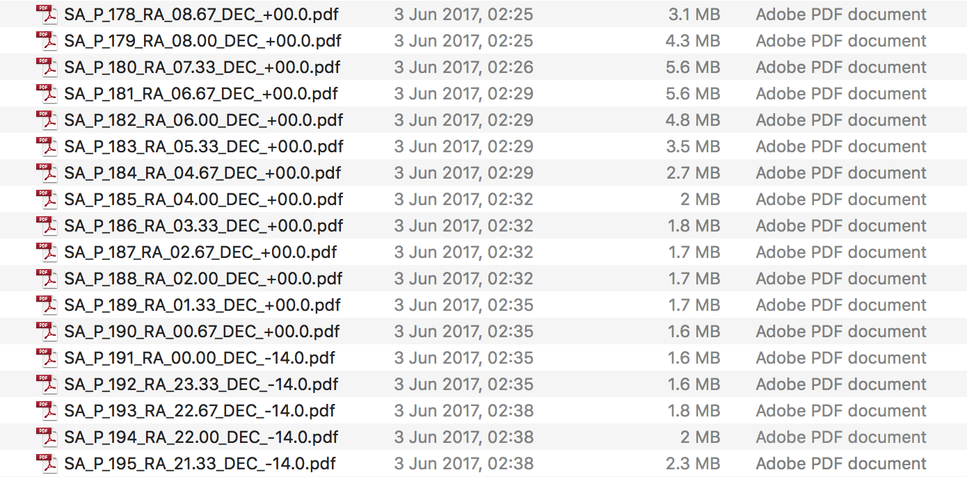
At the end I have a tidy ordered set of pages in the output folder. The size difference between the different pages shows nicely which pages have a larger number of objects plotted on them.
4. Sample pages and statistics
At the current stage, these are the numbers for the Leuven Star Atlas (for more details, see Section 3.3):
- Total number of stars: 361980 (down to and including magnitude 10.0)
- Variable stars: 6998
- Multiple (visual or physical) systems: 6411
- Total number of deep sky objects: 8690
- Galaxies: 6768
- Galaxy clusters: 29
- Globular clusters: 156
- Open clusters: 644
- Planetary nebulae: 742
- Bright nebulae: 154 (of which 134 have hand-drawn outlines – many of these actually cover multiple NGC objects, thus the total number of plotted catalog entries is higher)
- Dark nebulae: 197 (of which 163 have hand-drawn outlines)
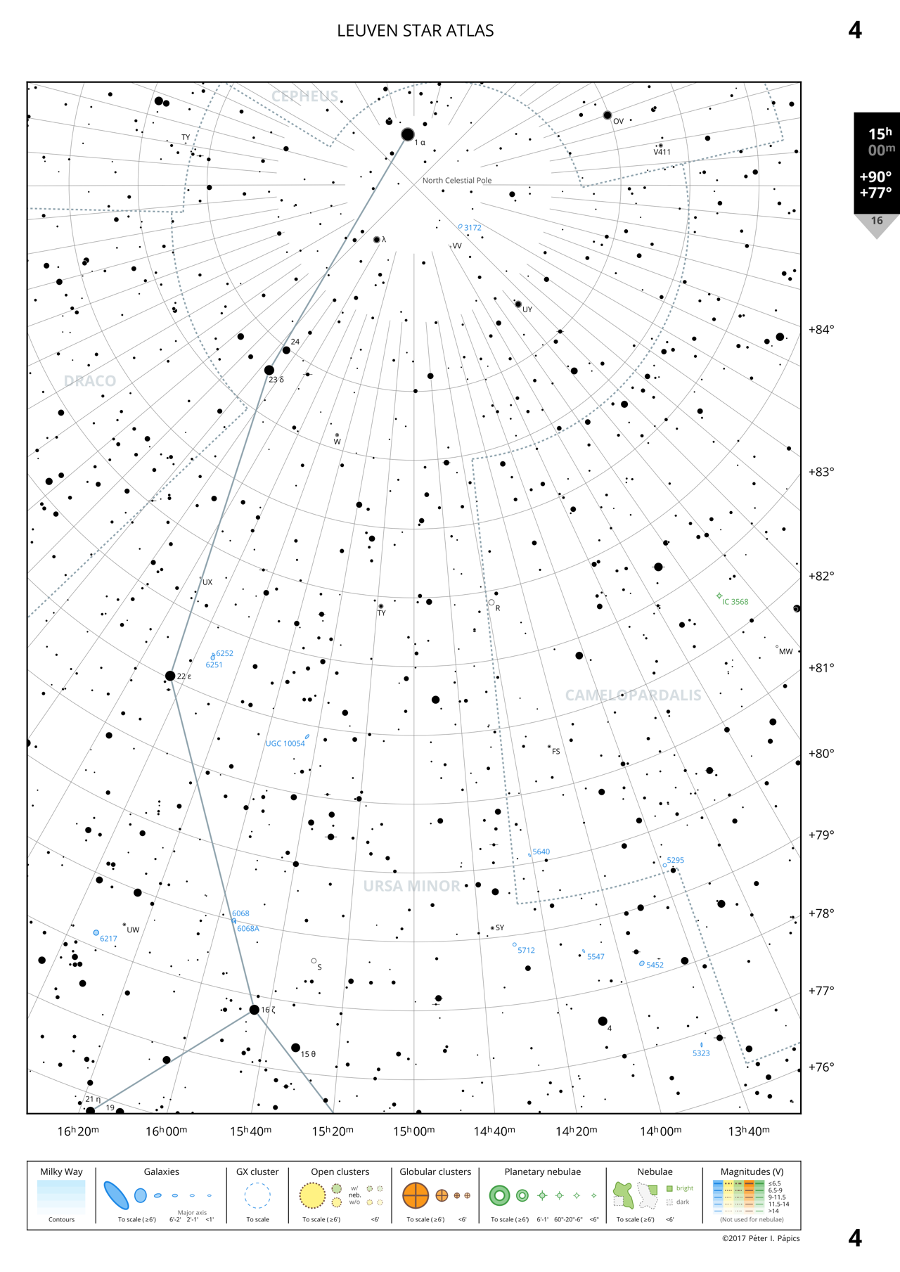
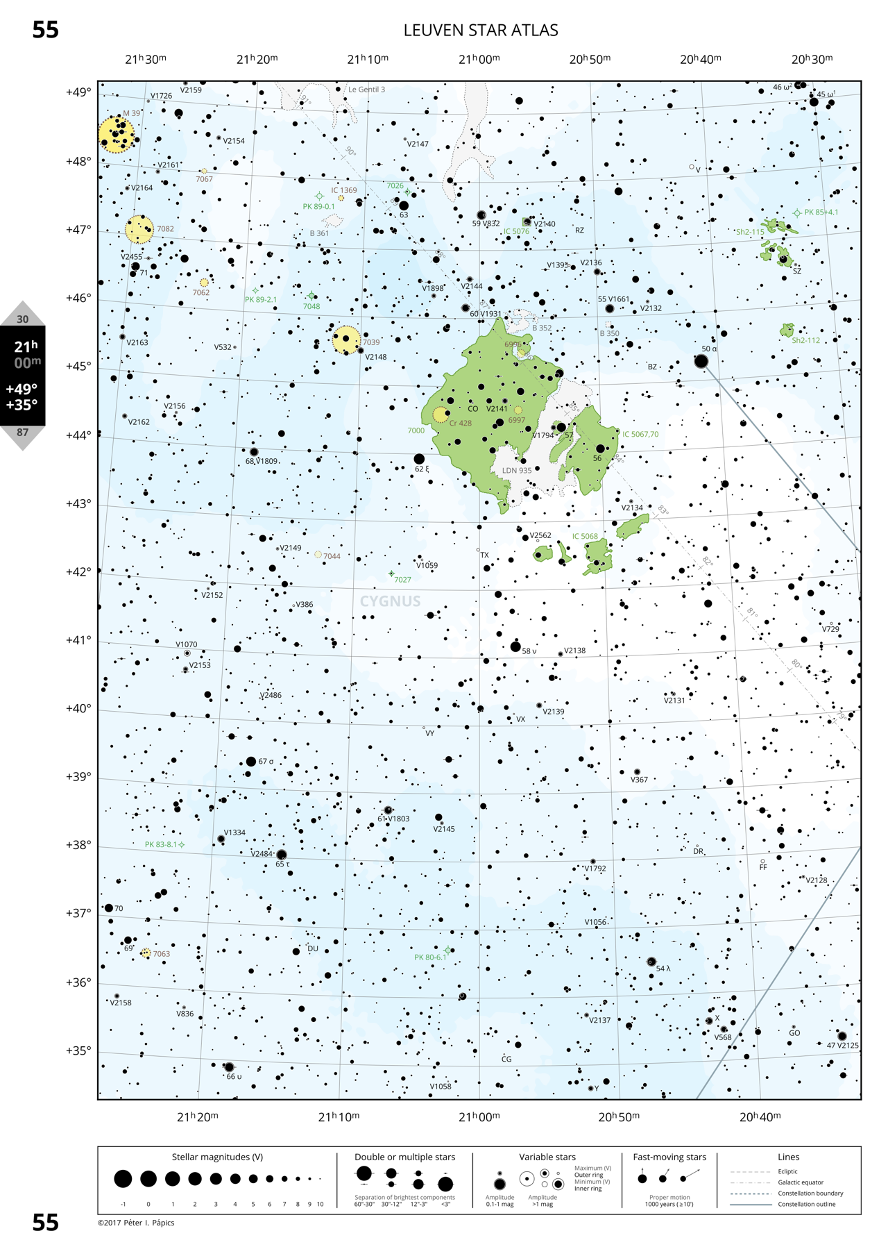
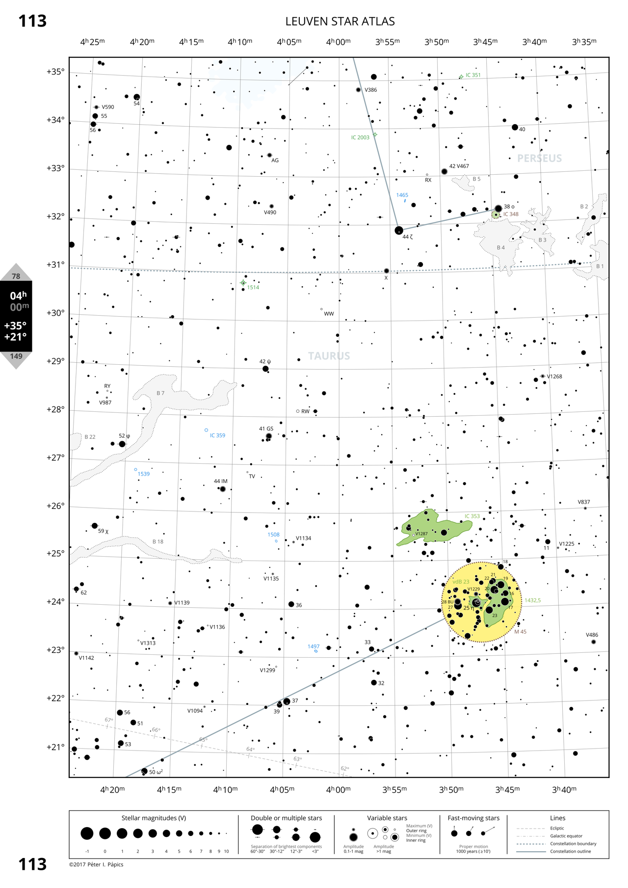
The full sky is displayed on 344 A4 pages (1.6 cm per degree of declination resolution), five of which can be downloaded in pdf by clicking on the example rasterised images below.
Page 4: Northern Ursa Minor
Page 55: Cygnus around NGC 7000 (North America Nebula)
Page 113: The Pleiades and the border of Taurus and Perseus
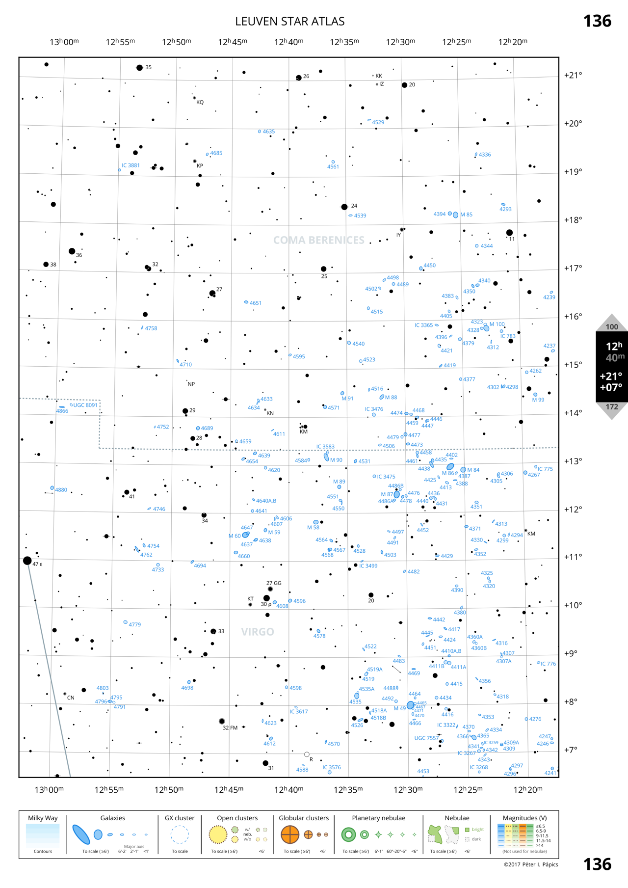
Page 136: Galaxies in Virgo and Coma Berenices
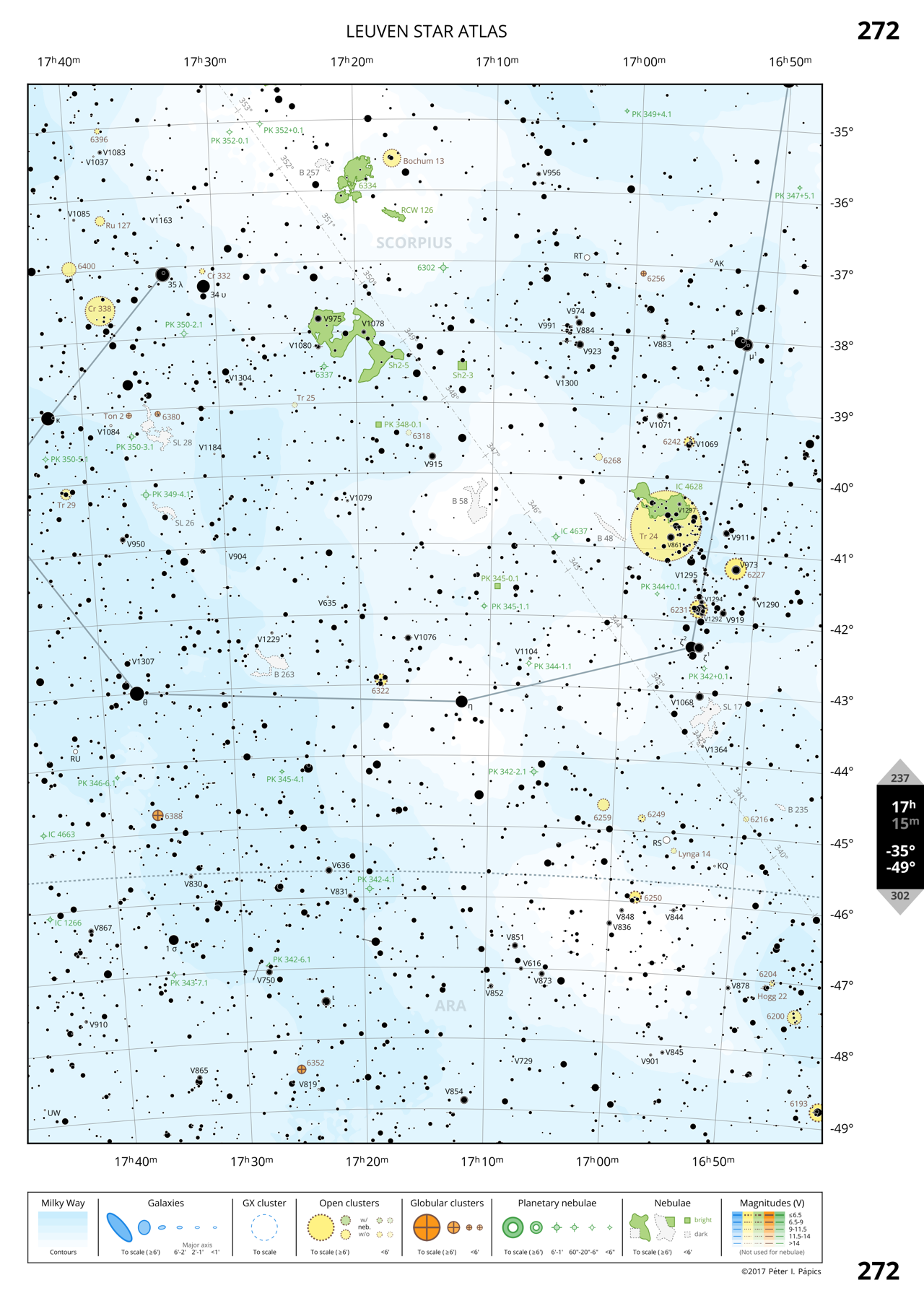
Page 272: Southern Scorpius
5. Future plans
The atlas is at a stage now where most of the larger work-packages are already completed, but there is still some work to be done before it can be printed into a nice book. A lot depends on whether I can actually get this published. I am determined to finish it and have a few copies printed in any case for myself and a few friends, but without an actual publication deadline, this will probably not happen next week, or the week after…
These are the components that are still missing or need completion:
- Labelling the remaining 339 pages. As mentioned earlier this could take me minimum 300 hours of work… (Or ~8 full time work weeks, or a year if I just do one page every day.)
- Close-up maps of selected dense regions: this means that I need to compile a stellar database down to ~11.0-11.5 magnitudes (press of a button, I do not need to change anything in my scripts), and implement a zoom-in factor (a scale multiplier that could be 2, 3, or 4), which I can use to modify, e.g., the field of view, and the cutoff sizes of deep sky objects. I could do this most likely in a day.
- Refinements in the deep sky object database: I still need to clean up a smaller mess in the Large and Small Magellanic Clouds, because I am not happy about the completeness of the database there (another day of work, but I have already drawn quite a few bright nebula there too), and I am also not satisfied with the number of galaxy clusters on the map right now, so I would like to extend that based on the original Abell+ data (I guess I could also do this in one or maximum two days). In general, a small extension might be necessary to the deep sky database in general, but this is up for some further considerations.
- Nicer constellation stick figures (as mentioned already earlier). This will take a bit longer (1-3 days), because I have to build a data file for this from scratch, and it is 100% manual work.
- Index charts: I need to create 6 pages (looking towards the poles, and the four cardinal directions) with a large field of view showing only the brightest stars, the constellations, and the borders of the fields covered by the individual atlas pages labelled with the page numbers, as these overview charts provide the basic navigation feature of any stellar atlas. To make this I need a stellar database down to ~5.5 magnitudes (press of a button), a function that draws the outline of the sky that is displayed on given atlas pages (maximum an hour of work), and some labelling, so in total this will not take more than a day again.
- An introduction chapter describing the use of the atlas, object types, etc. Also an index to the most interesting objects (Messier, Herschel 400, etc.) pointing to the atlas pages that contain them. This will probably be work for a week or two, since it includes quite some writing and brainstorming about what to write in the introduction.
- A nice cover page: I would like to have either something very classical, or a montage of a page of this atlas with a classical illustration of a constellation (from here). This design process will definitely take a few days too.
When all these points are crossed off the list, I will write another post to showcase the new features and the final atlas. Without the labelling work this could be done in less than a month, but I have holidays coming up, and soon I will also start looking for a new job, so I would not expect much before Christmas. Please if you have any remarks or suggestions, let me know in the comments section, I would highly appreciate it.


